Introduction
In this section, two machine learning models will be used to classify the vivo_ano3 column, Random Forest and XGBoost, for both datasets, São Paulo and other states.
The label is 1 if the patient is alive after three years of treatment and 0 if not.
The first approach is using the “raw data”, the second is without the EC column, the third one is without EC and HORMONIO, the fourth is using the grouped years and without the column EC and the fifth is also with the years gruped and without EC and HORMONIO.
The years will be grouped as follows: 2000 to 2003, 2004 to 2007, 2008 to 2011, 2012 to 2015 and 2016 until the end. So we will have 5 datasets for SP and another 5 for other states.
Reading the data from SP and other states.
We can see that we still have some missing values in both datasets, but the columns DTRECIDIVA, delta_t4, delta_t5 and delta_t6 will not be used in this approach.
[ ]:
df_SP = read_csv('/content/drive/MyDrive/Trabalho/Cancer/Datasets/geral_sp_labels.csv')
df_fora = read_csv('/content/drive/MyDrive/Trabalho/Cancer/Datasets/geral_fora_sp_labels.csv')
(506037, 77)
(32891, 77)
Here we have the correlations between the label and the other columns, the columns with higher correlations will not be used as features of the models, because they may have been used to create the label, such as the ULTINFO column, or they can be used as label for other machine learning models.
[ ]:
# SP
corr_matrix = df_SP.corr()
abs(corr_matrix['vivo_ano3']).sort_values(ascending = False).head(20)
vivo_ano3       1.000000
ULTIDIAG        0.746404
ULTICONS        0.740191
ULTITRAT        0.737903
vivo_ano5       0.688613
vivo_ano1       0.550659
obito_cancer    0.403906
obito_geral     0.365068
HORMONIO        0.236603
CIRURGIA        0.215579
MORFO           0.208184
ANODIAG         0.201279
ULTINFO         0.189965
QUIMIO          0.116880
G               0.103949
CLINICA         0.100960
DIAGTRAT        0.093799
SEXO            0.067311
TRATCONS        0.058532
CATEATEND       0.055419
Name: vivo_ano3, dtype: float64
[ ]:
# Other states
corr_matrix = df_fora.corr()
abs(corr_matrix['vivo_ano3']).sort_values(ascending = False).head(20)
vivo_ano3       1.000000
ULTIDIAG        0.759271
ULTICONS        0.753968
ULTITRAT        0.749534
vivo_ano5       0.667262
vivo_ano1       0.547481
obito_cancer    0.399038
obito_geral     0.385518
ANODIAG         0.258962
CIRURGIA        0.235109
ULTINFO         0.218422
HORMONIO        0.215508
MORFO           0.186335
CATEATEND       0.139831
QUIMIO          0.120061
TRATCONS        0.116820
DIAGTRAT        0.113094
RECLOCAL        0.060846
RECNENHUM       0.059315
SEXO            0.059252
Name: vivo_ano3, dtype: float64
Here we have the number of examples for each category of the label, it is clear that there is an imbalance, similar to the previous classification.
[ ]:
df_SP.vivo_ano3.value_counts()
0    260942
1    245095
Name: vivo_ano3, dtype: int64
[ ]:
df_fora.vivo_ano3.value_counts()
0    17264
1    15627
Name: vivo_ano3, dtype: int64
Years of diagnosis present in the data.
[ ]:
np.sort(df_SP.ANODIAG.unique())
array([2000, 2001, 2002, 2003, 2004, 2005, 2006, 2007, 2008, 2009, 2010,
       2011, 2012, 2013, 2014, 2015, 2016, 2017, 2018, 2019, 2020, 2021])
[ ]:
np.sort(df_fora.ANODIAG.unique())
array([2000, 2001, 2002, 2003, 2004, 2005, 2006, 2007, 2008, 2009, 2010,
       2011, 2012, 2013, 2014, 2015, 2016, 2017, 2018, 2019, 2020])
Before dividing the datasets, it is necessary to select only the patients who have been followed up for at least three years.
[ ]:
# SP
df_SP_ano3 = df_SP[~((df_SP.obito_geral == 0) & (df_SP.vivo_ano3 == 0))]
df_SP_ano3.shape
(409182, 77)
[ ]:
# Other States
df_fora_ano3 = df_fora[~((df_fora.obito_geral == 0) & (df_fora.vivo_ano3 == 0))]
df_fora_ano3.shape
(25280, 77)
First approach
Approach with “raw data”.
Preprocessing
Now we are going to divide the data into training and testing, and then do the preprocessing in both datasets to perform the training of the models and their evaluation.
First, it is necessary to define the columns that will be used as features and the label. We will not use some columns of the datasets: UFRESID, because we already have the division between SP and other states in the two datasets.
It was chosen to keep the column IDADE, so we will not use the FAIXAETAR. Finally, the other columns contained in the list list_drop are possible labels, so they will not be used as features for machine learning models.
[ ]:
list_drop = ['UFRESID', 'FAIXAETAR', 'ULTICONS', 'ULTIDIAG', 'ULTITRAT',
             'obito_geral', 'obito_cancer', 'vivo_ano1', 'vivo_ano5', 'ULTINFO']

# 'RECNENHUM', 'RECLOCAL', 'RECREGIO', 'REC01', 'REC02', 'REC03', 'RECDIST'

lb = 'vivo_ano3'
A function was created to perform the preprocessing, preprocessing, that uses the other functions created, get_train_test (divides the dataset into train and test sets), train_preprocessing (do the preprocessing of the train set) and test_preprocessing (do the preprocessing of the test set).
To see the complete function go to the functions section.
SP
[ ]:
X_train_SP, X_test_SP, y_train_SP, y_test_SP, feat_cols_SP = preprocessing(df_SP_ano3, list_drop, lb,
                                                                           random_state=seed,
                                                                           balance_data=False,
                                                                           encoder_type='LabelEncoder',
                                                                           norm_name='StandardScaler')
X_train = (306886, 66), X_test = (102296, 66)
y_train = (306886,), y_test = (102296,)
Other states
[ ]:
X_train_OS, X_test_OS, y_train_OS, y_test_OS, feat_cols_OS = preprocessing(df_fora_ano3, list_drop, lb,
                                                                           random_state=seed,
                                                                           balance_data=False,
                                                                           encoder_type='LabelEncoder',
                                                                           norm_name='StandardScaler')
X_train = (18960, 66), X_test = (6320, 66)
y_train = (18960,), y_test = (6320,)
Training machine learning models
After dividing the data into training and testing, using the encoder and normalizing, the data is ready to be used by the machine learning models.
Random Forest
The first model that will be tested is the Random Forest, for this test the parameter random_state will be used, to obtain the same training values of the model every time it is runned.
The hyperparameter class_weight was also used, because the model has difficulty learning the class with fewer examples, so using this parameter this class will have a higher weight in the training of the model.
[ ]:
# SP
rf_sp = RandomForestClassifier(class_weight={0:1.557, 1:1},
                               random_state=seed,
                               criterion='entropy',
                               max_depth=10)

rf_sp.fit(X_train_SP, y_train_SP)
RandomForestClassifier(class_weight={0: 1.557, 1: 1}, criterion='entropy',
                       max_depth=10, random_state=10)
[ ]:
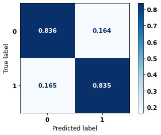
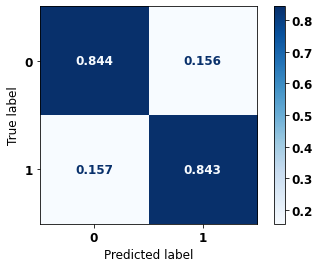
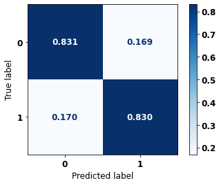
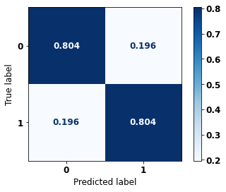
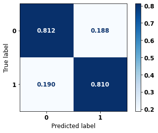
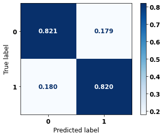
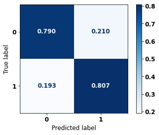
display_confusion_matrix(rf_sp, X_test_SP, y_test_SP)

              precision    recall  f1-score   support

           0      0.740     0.810     0.773     41022
           1      0.864     0.809     0.836     61274

    accuracy                          0.809    102296
   macro avg      0.802     0.809     0.804    102296
weighted avg      0.814     0.809     0.811    102296
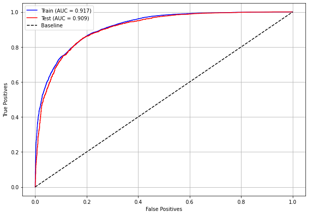
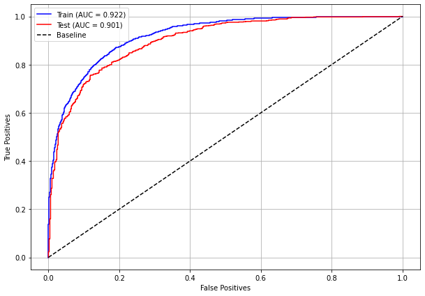
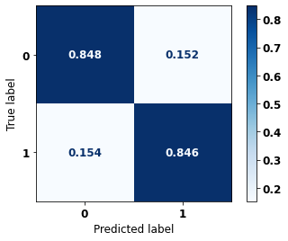
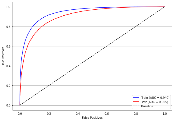
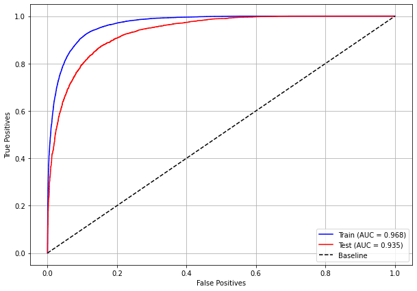
The confusion matrix obtained for the Random Forest, with SP data, shows a good performance of the model, with 81% of accuracy.
[ ]:
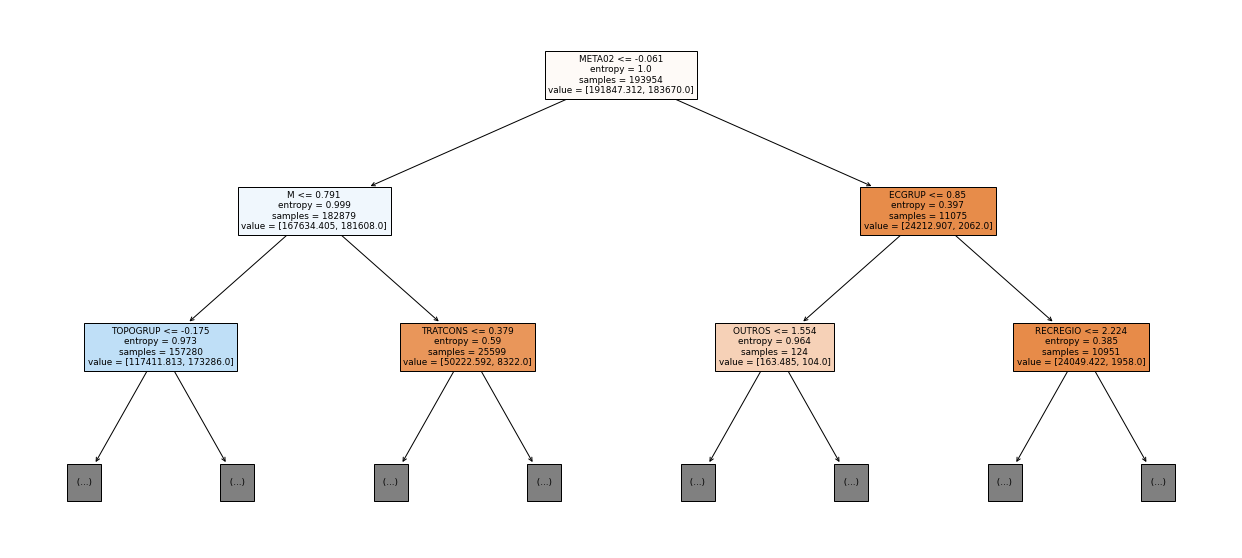
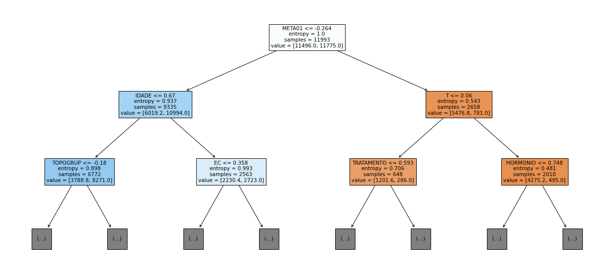
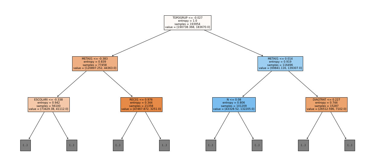
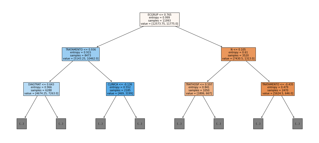
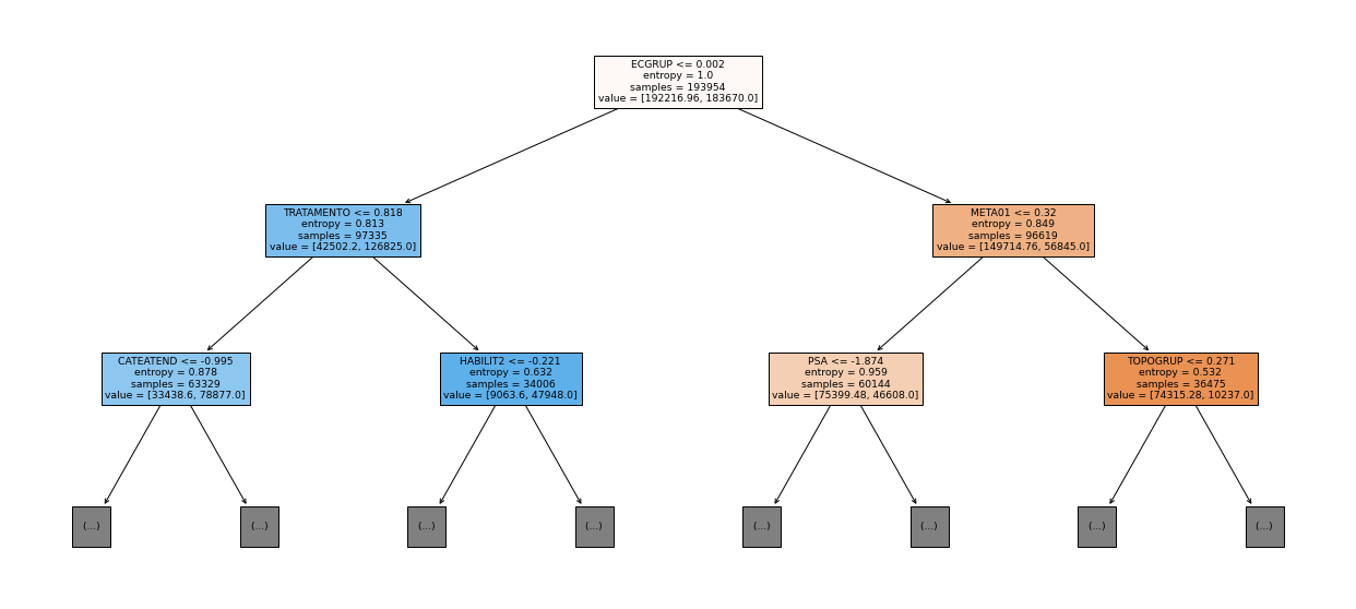
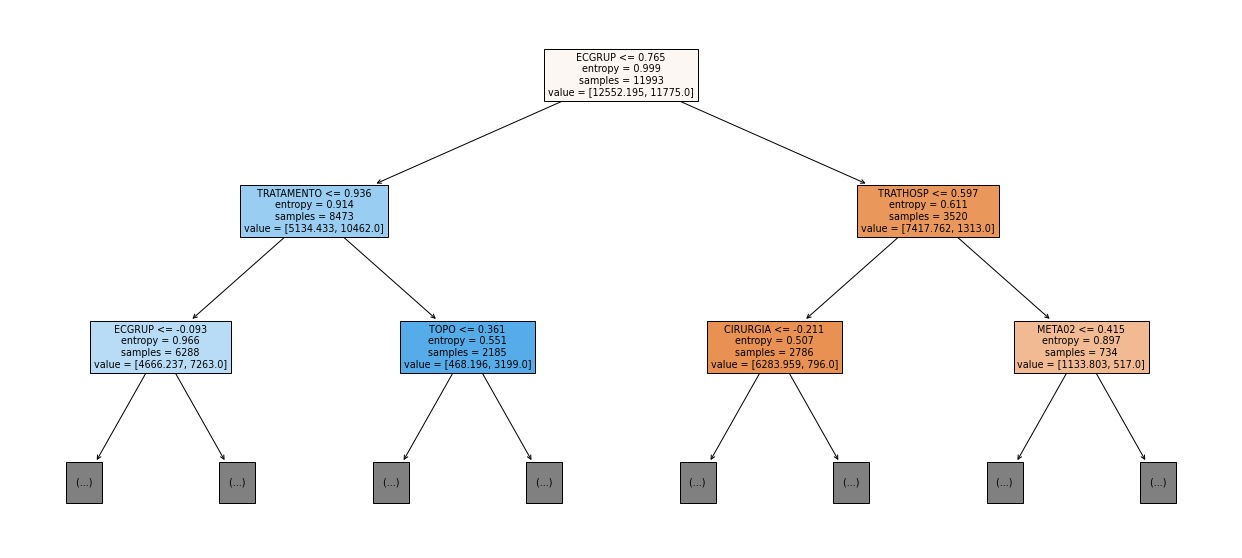
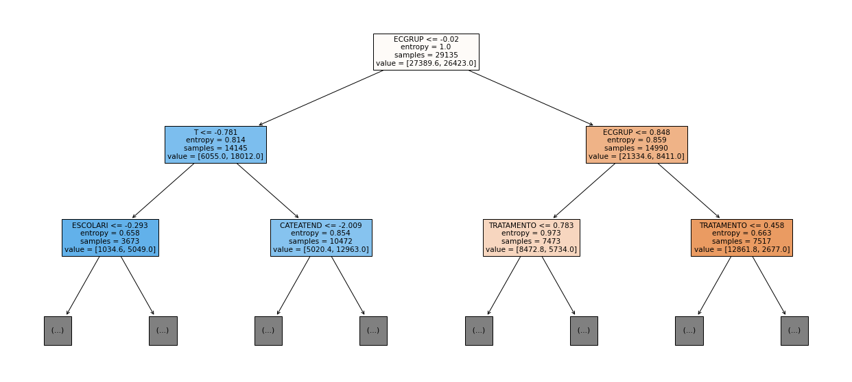
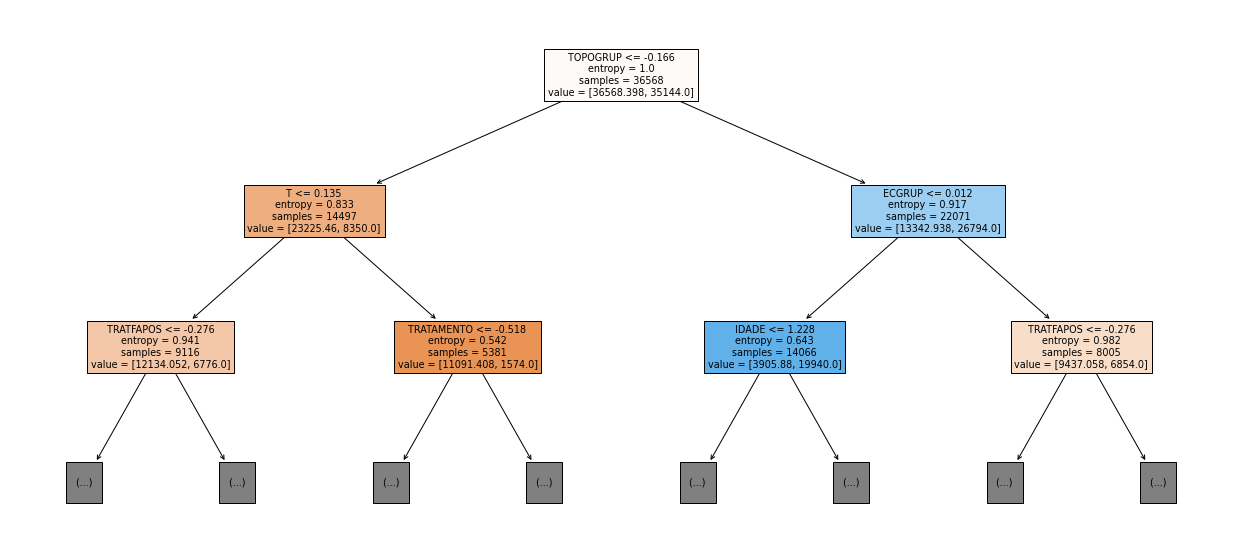
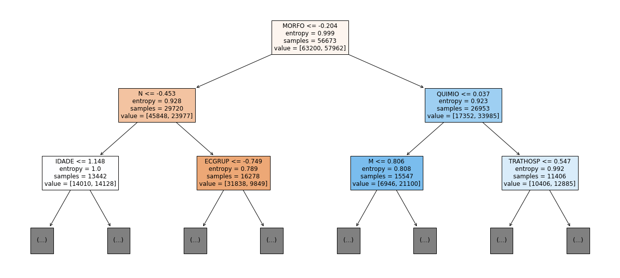
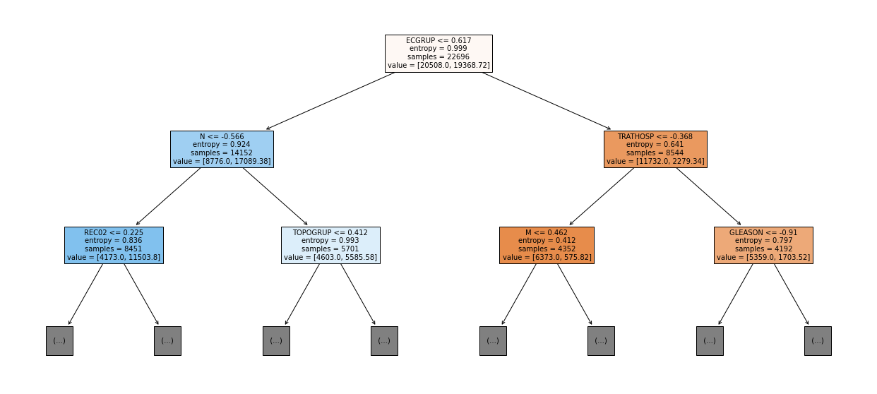
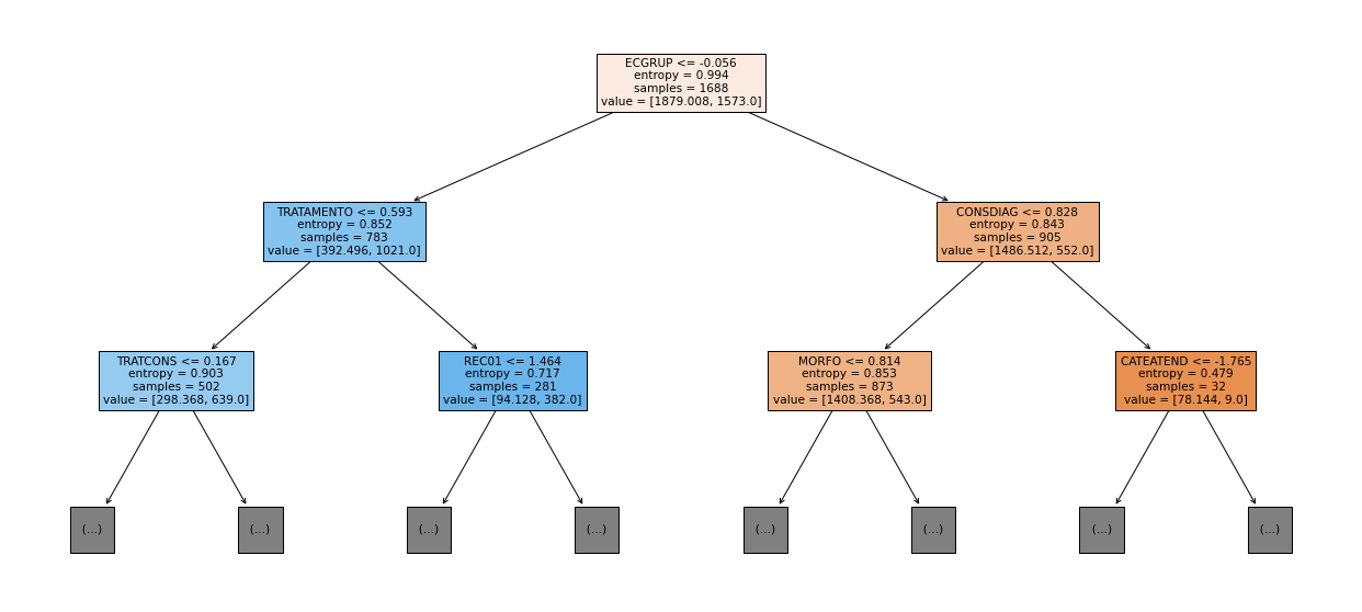
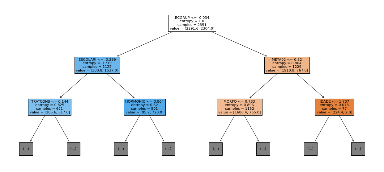
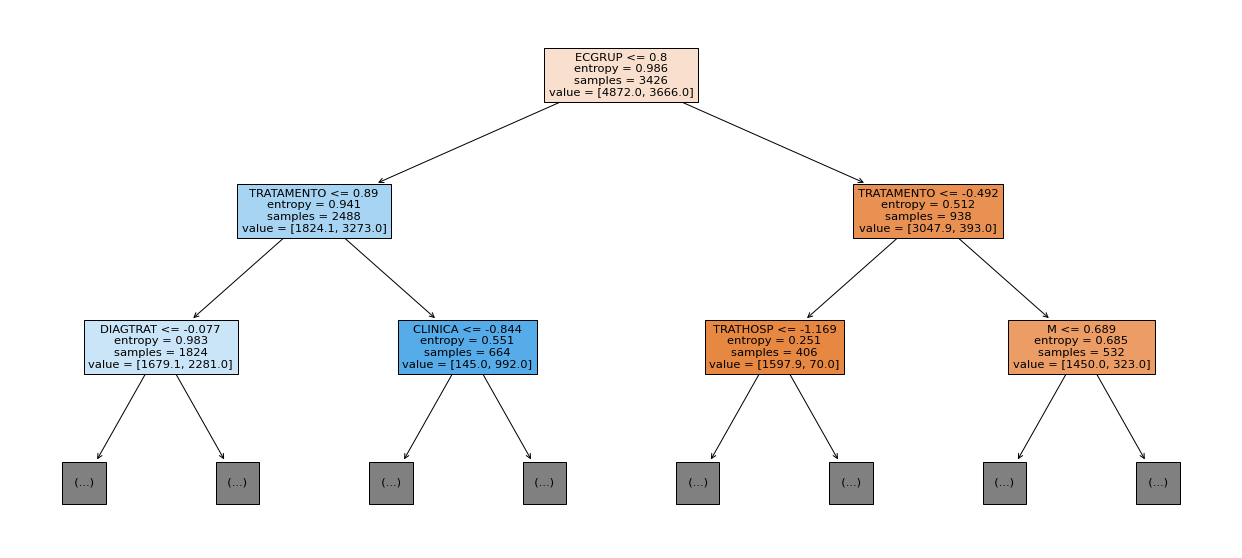
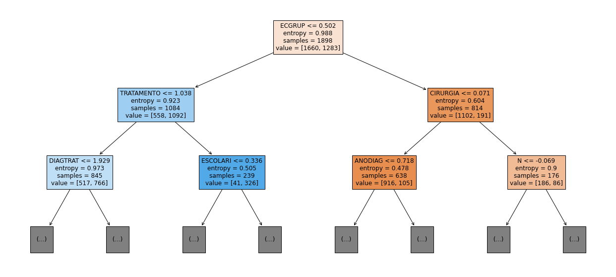
show_tree(rf_sp, feat_cols_SP, 2)
[ ]:
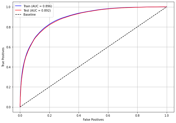
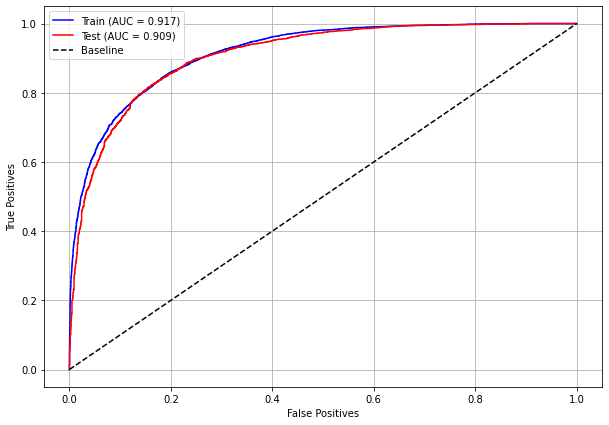
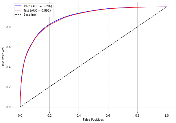
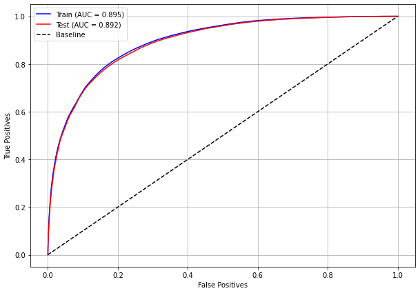
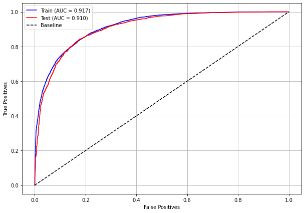
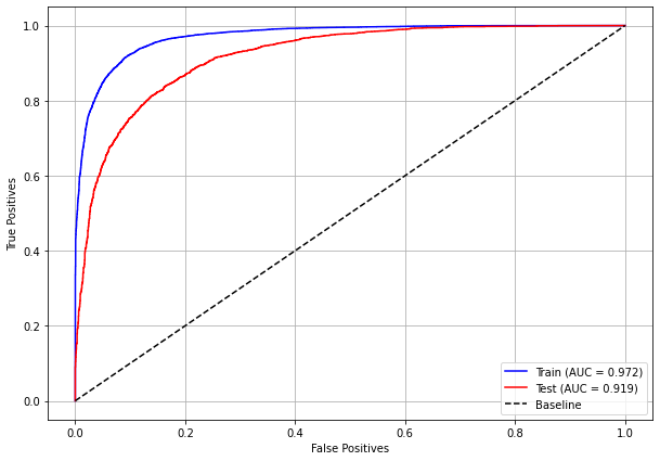
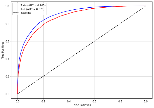
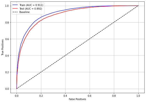
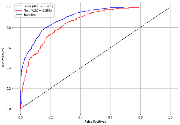
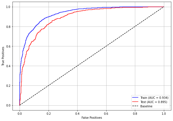
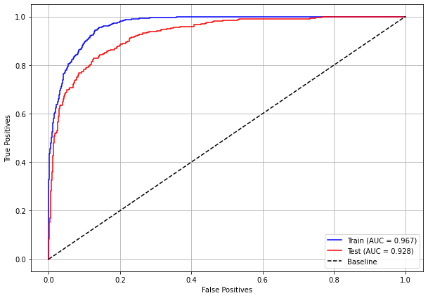
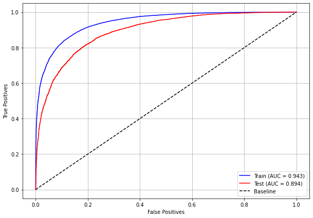
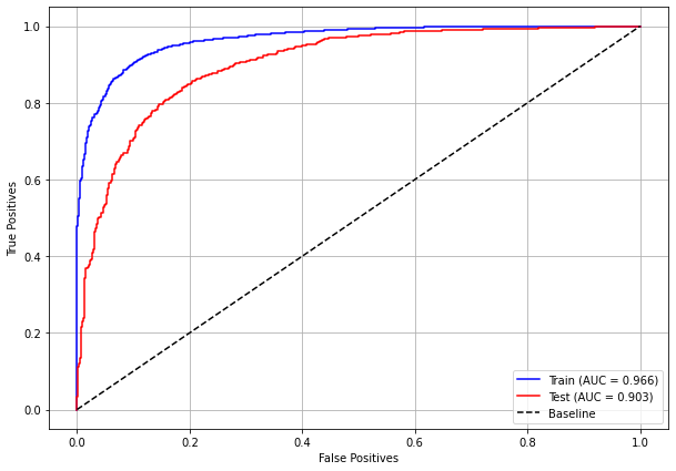
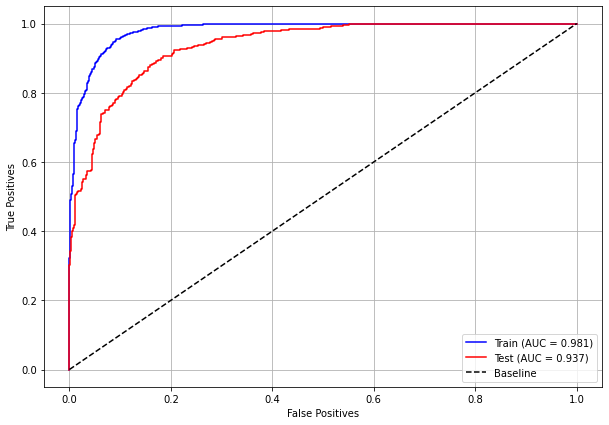
plot_roc_curve(rf_sp, X_train_SP, X_test_SP, y_train_SP, y_test_SP)
[ ]:
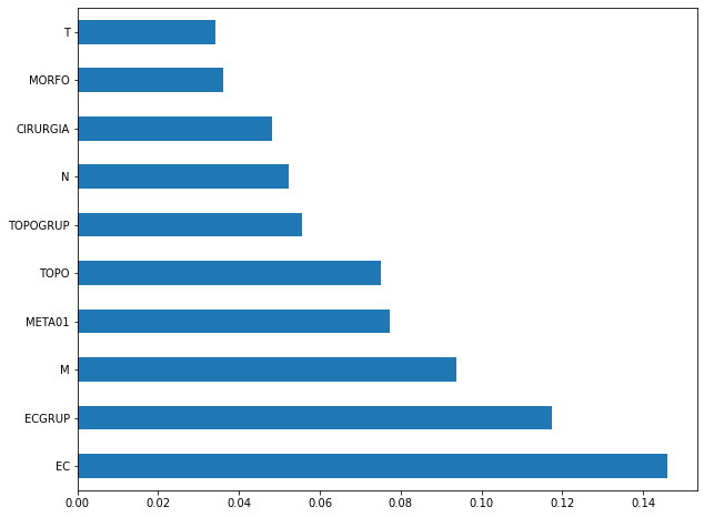
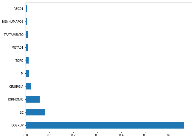
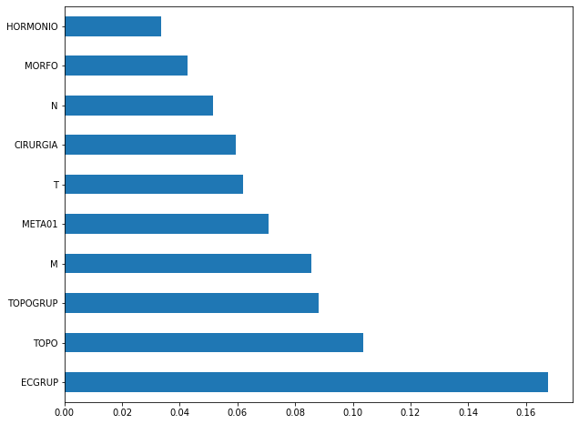
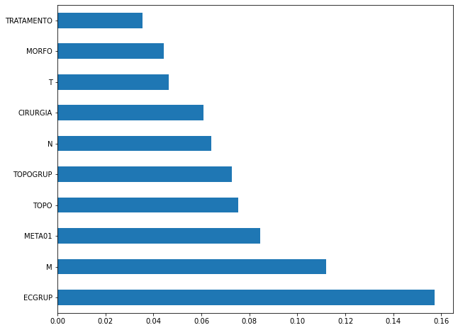
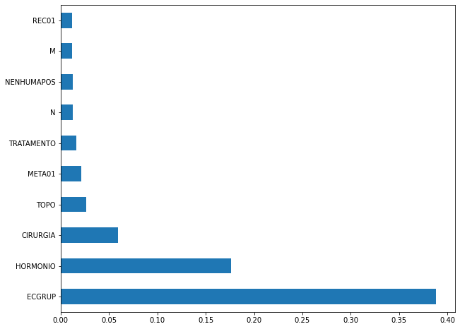
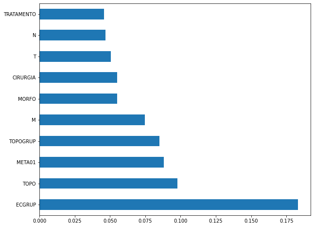
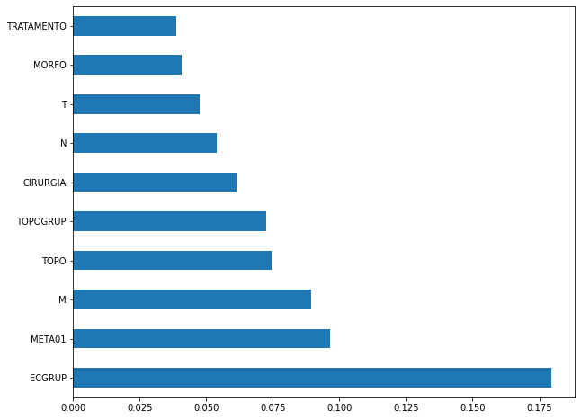
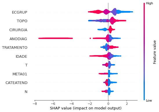
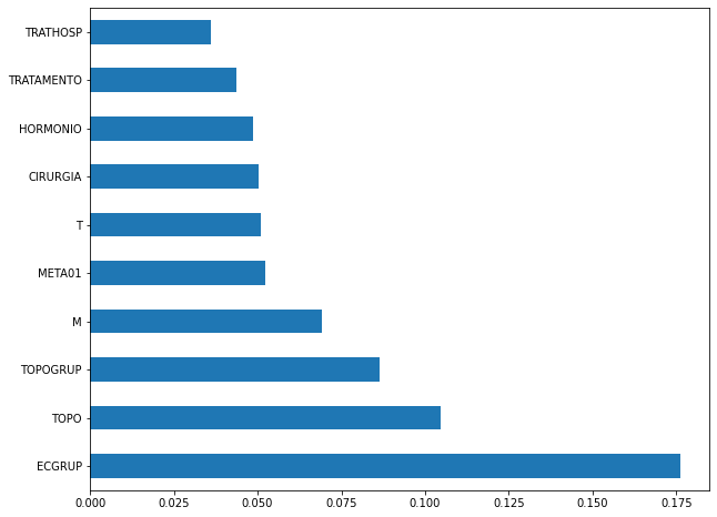
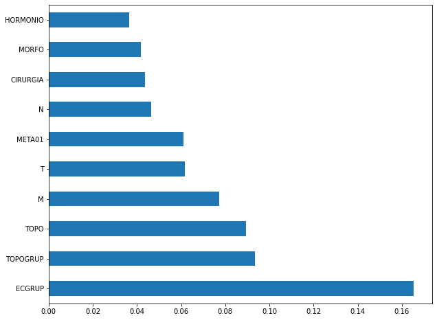
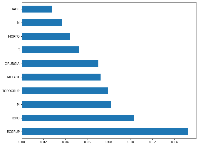
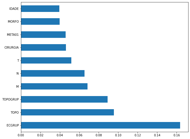
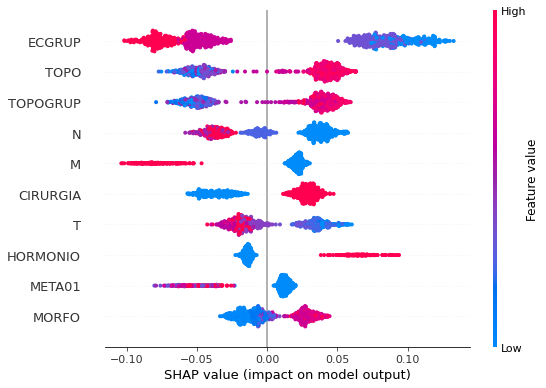
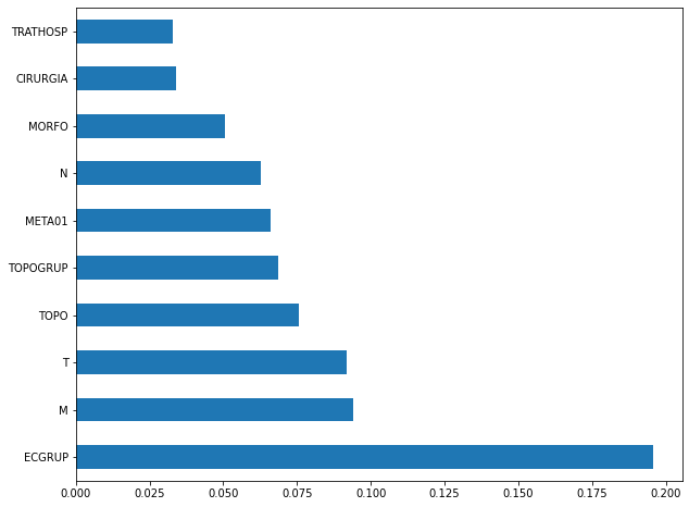
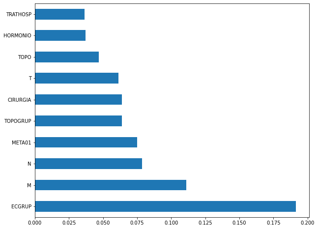
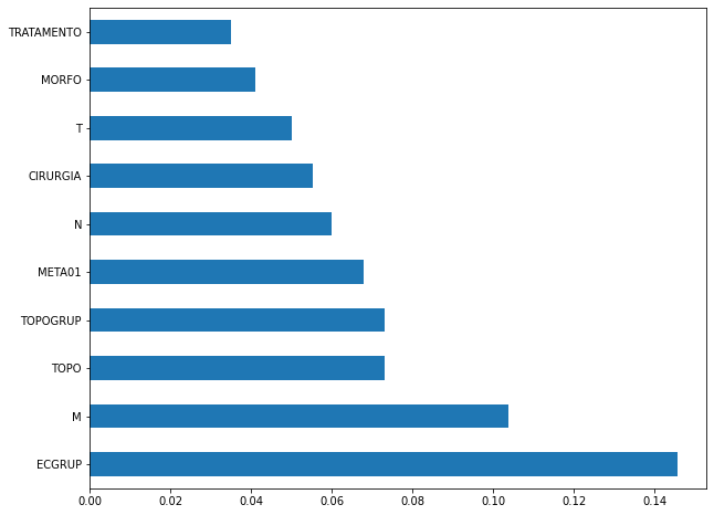
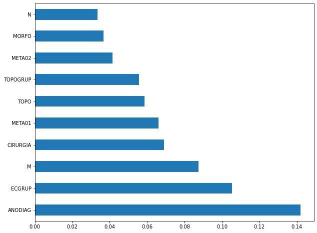
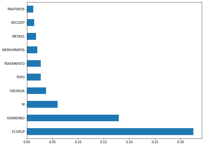
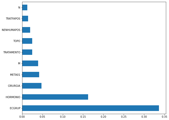
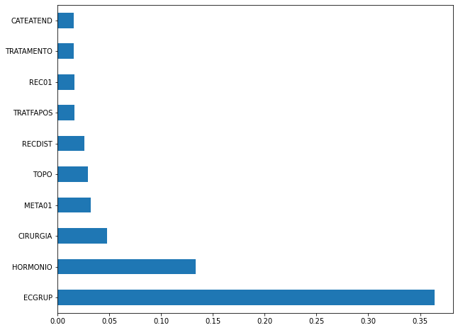
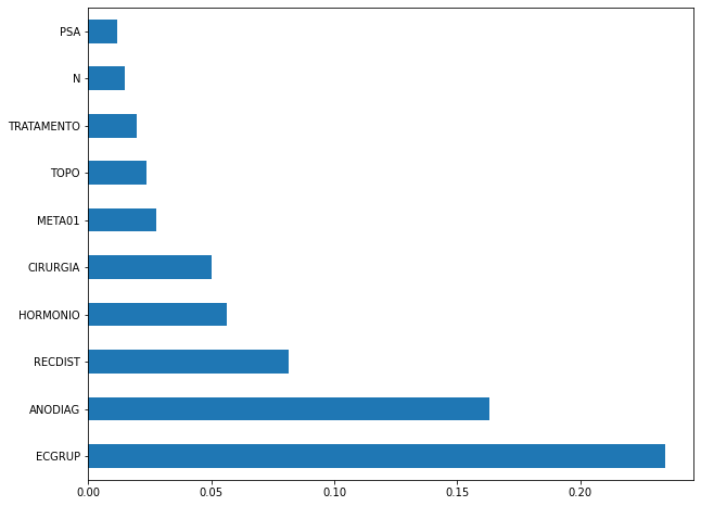
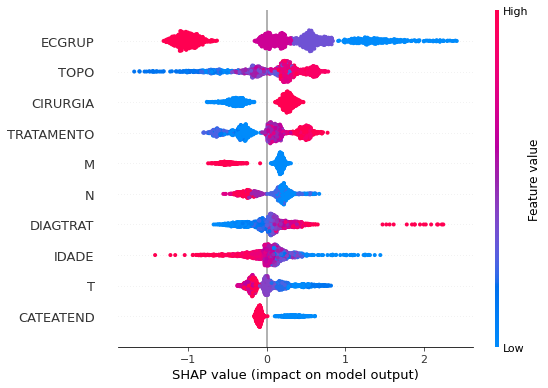
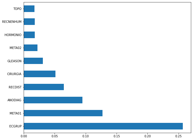
plot_feat_importances(rf_sp, feat_cols_SP)
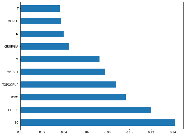
The four most important features in the model were
EC,ECGRUP,TOPOandTOPOGRUP.
[ ]:
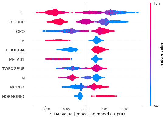
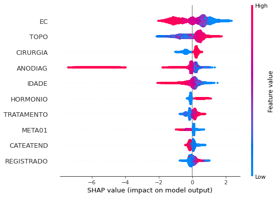
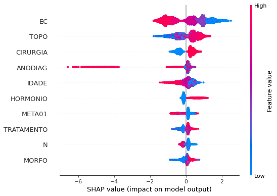
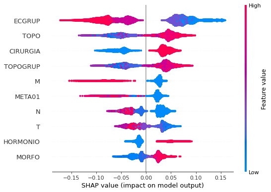
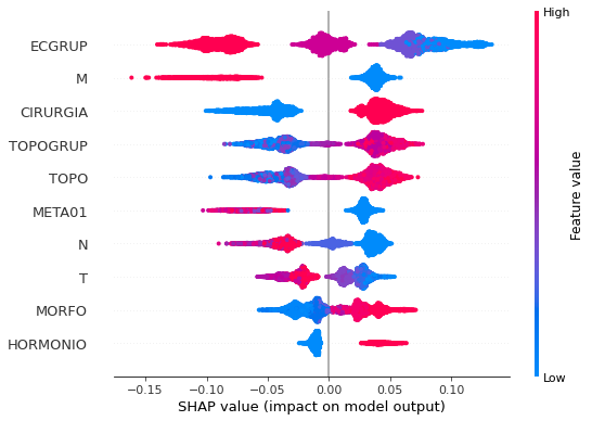
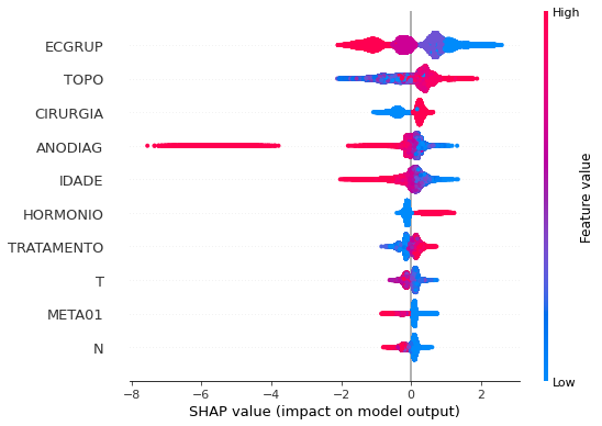
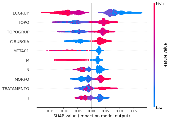
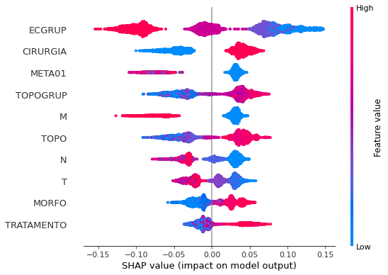
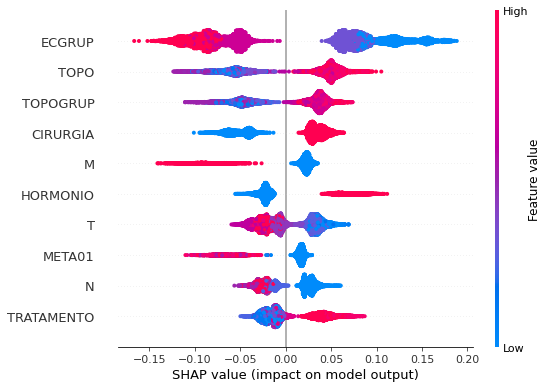
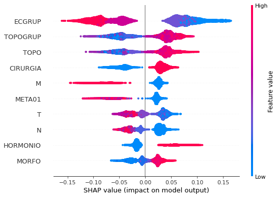
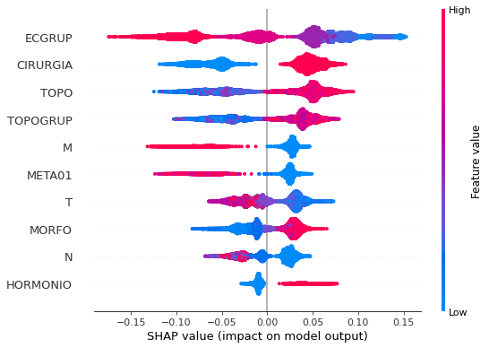
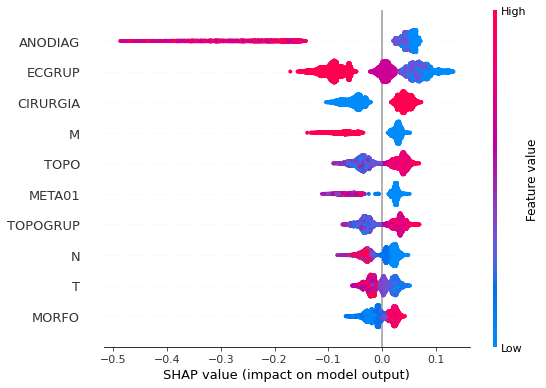
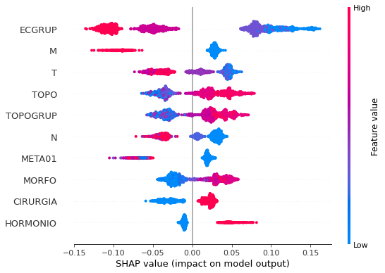
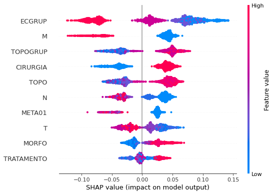
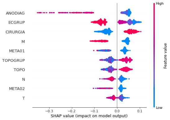
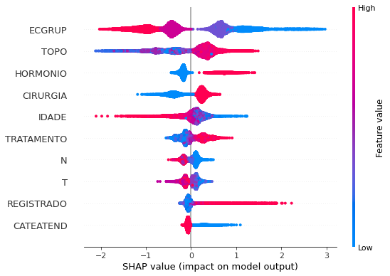
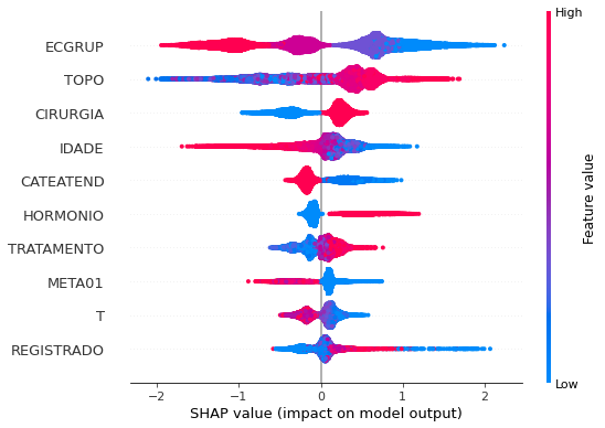
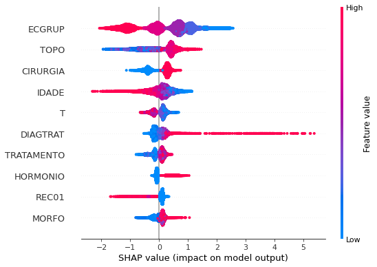
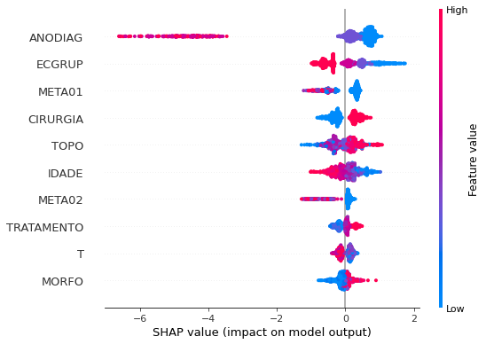
plot_shap_values(rf_sp, X_test_SP, feat_cols_SP)
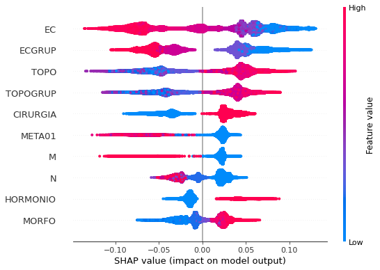
Note that larger values of the EC column, shown in pink, have more influence for the model’s prediction to be class 0, smaller values have greater weight for the prediction to be class 1. This behavior was expected, because the higher the clinical stage, worse is the stage of cancer.
The other columns shown follow the same logic.
[ ]:
# Other states
rf_fora = RandomForestClassifier(class_weight={0:1.6, 1:1},
                                 random_state=seed,
                                 criterion='entropy',
                                 max_depth=8)

rf_fora.fit(X_train_OS, y_train_OS)
RandomForestClassifier(class_weight={0: 1.6, 1: 1}, criterion='entropy',
                       max_depth=8, random_state=10)
[ ]:
display_confusion_matrix(rf_fora, X_test_OS, y_test_OS)

              precision    recall  f1-score   support

           0      0.750     0.829     0.788      2413
           1      0.887     0.830     0.857      3907

    accuracy                          0.829      6320
   macro avg      0.819     0.829     0.823      6320
weighted avg      0.835     0.829     0.831      6320
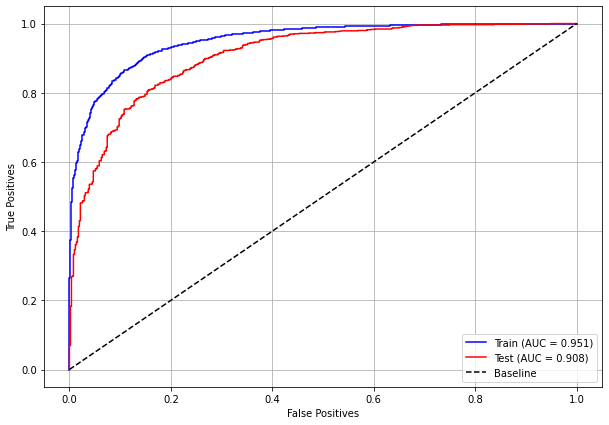
The confusion matrix obtained for the Random Forest algorithm, with other states data, shows a good performance of the model, because the model achieves a 83% of accuracy.
[ ]:
show_tree(rf_fora, feat_cols_OS, 2)
[ ]:
plot_roc_curve(rf_fora, X_train_OS, X_test_OS, y_train_OS, y_test_OS)
[ ]:
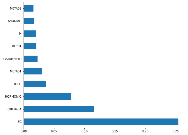
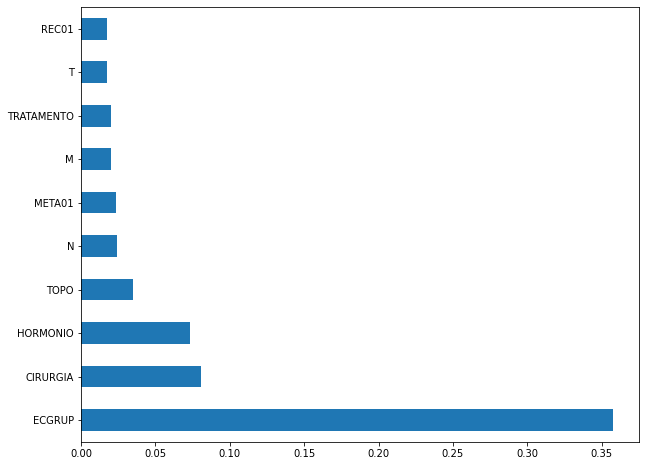
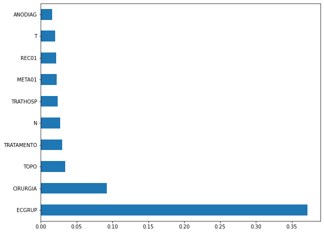
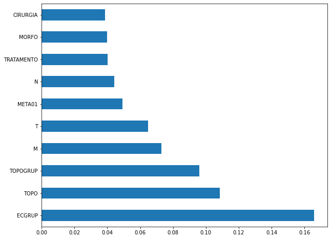
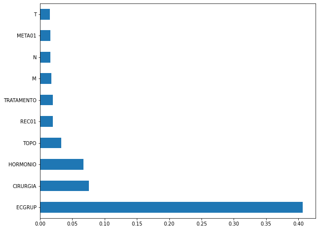
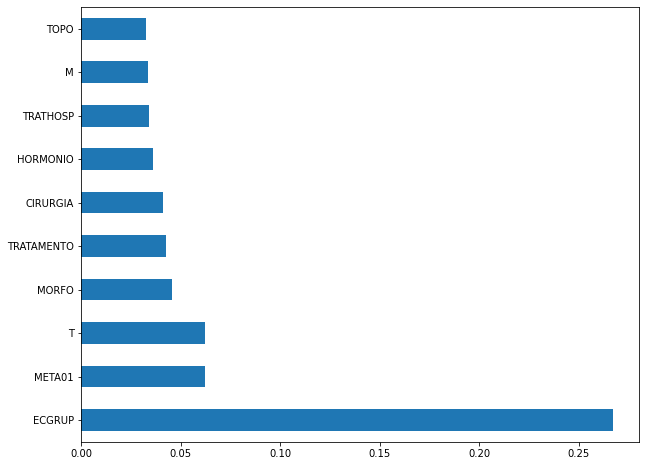
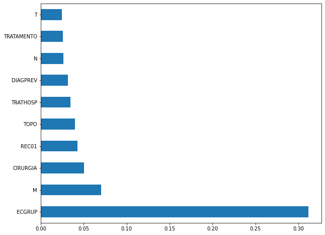
plot_feat_importances(rf_fora, feat_cols_OS)
The four most important features in the model were
EC,ECGRUP,MandMETA01.
[ ]:
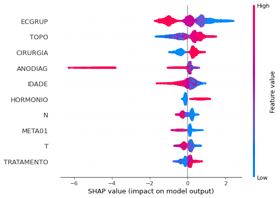
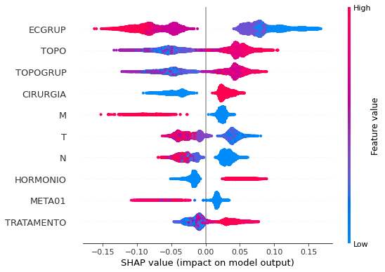
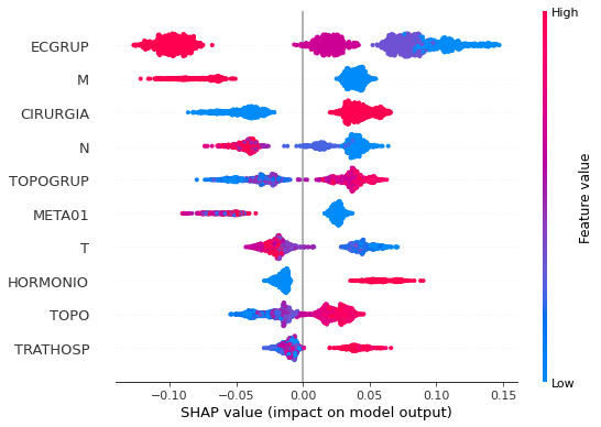
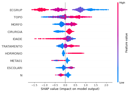
plot_shap_values(rf_fora, X_test_OS, feat_cols_OS)
Note that larger values of the EC column, shown in pink, have more influence for the model’s prediction to be class 0, smaller values have greater weight for the prediction to be class 1. This behavior was expected, because the higher the clinical stage, worse is the stage of cancer.
The other columns shown follow the same logic.
Randomized Grid Search
[ ]:
# RandomizedSearchCV
hyperRF = {'n_estimators': [100, 150, 200, 250],
           'max_depth': [5, 8, 10, 12, 15],
           'min_samples_split': [2, 5, 10, 15],
           'min_samples_leaf': [1, 2, 5, 10]}

rf = RandomForestClassifier(random_state=seed, criterion='entropy')

randRS = RandomizedSearchCV(rf, hyperRF, n_iter=20, cv=5, n_jobs=-1,
                            random_state=seed)
[ ]:
# SP
bestSP = randRS.fit(X_train_SP, y_train_SP)
[ ]:
bestSP.best_params_
{'n_estimators': 200,
 'min_samples_split': 10,
 'min_samples_leaf': 2,
 'max_depth': 15}
[ ]:
# SP
rf_sp_opt = bestSP.best_estimator_
rf_sp_opt.set_params(class_weight={0:1.61, 1:1})

rf_sp_opt.fit(X_train_SP, y_train_SP)
RandomForestClassifier(class_weight={0: 1.61, 1: 1}, criterion='entropy',
                       max_depth=15, min_samples_leaf=2, min_samples_split=10,
                       n_estimators=200, random_state=10)
[ ]:
display_confusion_matrix(rf_sp_opt, X_test_SP, y_test_SP)

              precision    recall  f1-score   support

           0      0.753     0.820     0.785     41022
           1      0.872     0.820     0.845     61274

    accuracy                          0.820    102296
   macro avg      0.813     0.820     0.815    102296
weighted avg      0.824     0.820     0.821    102296
[ ]:
# Other States
bestOS = randRS.fit(X_train_OS, y_train_OS)
[ ]:
bestOS.best_params_
{'n_estimators': 200,
 'min_samples_split': 10,
 'min_samples_leaf': 2,
 'max_depth': 15}
[ ]:
# Other states
rf_fora_opt = bestOS.best_estimator_
rf_fora_opt.set_params(class_weight={0:2.06, 1:1})

rf_fora_opt.fit(X_train_OS, y_train_OS)
RandomForestClassifier(class_weight={0: 2.06, 1: 1}, criterion='entropy',
                       max_depth=15, min_samples_leaf=2, min_samples_split=10,
                       n_estimators=200, random_state=10)
[ ]:
display_confusion_matrix(rf_fora_opt, X_test_OS, y_test_OS)

              precision    recall  f1-score   support

           0      0.765     0.840     0.801      2413
           1      0.895     0.841     0.867      3907

    accuracy                          0.840      6320
   macro avg      0.830     0.840     0.834      6320
weighted avg      0.845     0.840     0.842      6320
XGBoost
The training of the XGBoost model follows the same pattern with random_state. A higher weight was also used for the class with fewer examples, using the hyperparameter scale_pos_weight.
The hyperparameter max_depth was chosen as 10 because the default value for this hyperparameter is 3, a low value for the amount of data we have.
[ ]:
# SP
xgboost_sp = XGBClassifier(max_depth=10,
                               scale_pos_weight=0.651,
                               random_state=seed)

xgboost_sp.fit(X_train_SP, y_train_SP)
XGBClassifier(max_depth=10, random_state=10, scale_pos_weight=0.651)
[ ]:
display_confusion_matrix(xgboost_sp, X_test_SP, y_test_SP)

              precision    recall  f1-score   support

           0      0.767     0.830     0.798     41022
           1      0.880     0.831     0.855     61274

    accuracy                          0.831    102296
   macro avg      0.824     0.831     0.826    102296
weighted avg      0.835     0.831     0.832    102296
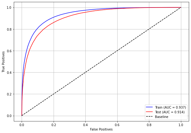
The confusion matrix obtained for the XGBoost, with SP data, shows a good performance of the model, with 83% of accuracy.
[ ]:
plot_roc_curve(xgboost_sp, X_train_SP, X_test_SP, y_train_SP, y_test_SP)

[ ]:
plot_feat_importances(xgboost_sp, feat_cols_SP)
The four most important features in the model were
ECGRUP,EC,HORMONIOandCIRURGIA.
[ ]:
plot_shap_values(xgboost_sp, X_test_SP, feat_cols_SP)
Note that larger values of the EC column, shown in pink, have more influence for the model’s prediction to be class 0, smaller values have greater weight for the prediction to be class 1. This behavior was expected, because the higher the clinical stage, worse is the stage of cancer.
The other columns shown follow the same logic.
[ ]:
# Other states
xgboost_fora = XGBClassifier(max_depth=8,
                             scale_pos_weight=0.55,
                             random_state=seed)

xgboost_fora.fit(X_train_OS, y_train_OS)
XGBClassifier(max_depth=8, random_state=10, scale_pos_weight=0.55)
[ ]:
display_confusion_matrix(xgboost_fora, X_test_OS, y_test_OS)
              precision    recall  f1-score   support

           0      0.758     0.836     0.795      2413
           1      0.892     0.835     0.863      3907

    accuracy                          0.836      6320
   macro avg      0.825     0.836     0.829      6320
weighted avg      0.841     0.836     0.837      6320
The confusion matrix obtained for the XGBoost algorithm, with other states data, shows a good performance of the model, because the model achieves a 84% of accuracy.
[ ]:
plot_roc_curve(xgboost_fora, X_train_OS, X_test_OS, y_train_OS, y_test_OS)

[ ]:
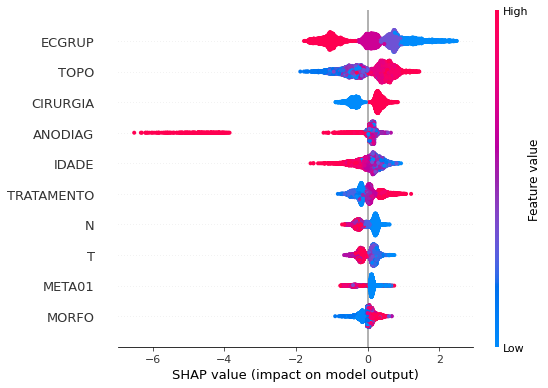
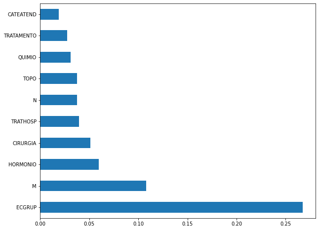
plot_feat_importances(xgboost_fora, feat_cols_OS)
The four most important features in the model were
EC,CIRURGIA,HORMONIOandTOPO.
[ ]:
plot_shap_values(xgboost_fora, X_test_OS, feat_cols_OS)
Note that larger values of the EC column, shown in pink, have more influence for the model’s prediction to be class 0, smaller values have greater weight for the prediction to be class 1. This behavior was expected, because the higher the clinical stage, worse is the stage of cancer.
The other columns shown follow the same logic.
Randomized Grid Search
[ ]:
# RandomizedSearchCV
hyperXGB = {'learning_rate': [0.05, 0.10, 0.15, 0.20],
            'max_depth': [5, 8, 10, 12, 15],
            'min_child_weight': [1, 3, 5, 7],
            'gamma': [0.0, 0.1, 0.2 , 0.3],
            'colsample_bytree': [0.3, 0.4, 0.5, 0.7],
            'n_estimators': [100, 150, 200, 250]}

xgboost = XGBClassifier(random_state=seed)
xgbRS = RandomizedSearchCV(xgboost, hyperXGB, n_iter=20, cv=5, n_jobs=-1,
                           random_state=seed)
[ ]:
# SP
bestSP = xgbRS.fit(X_train_SP, y_train_SP)
[ ]:
bestSP.best_params_
{'n_estimators': 250,
 'min_child_weight': 5,
 'max_depth': 10,
 'learning_rate': 0.15,
 'gamma': 0.3,
 'colsample_bytree': 0.4}
[ ]:
# SP
xgb_sp_opt = bestSP.best_estimator_
xgb_sp_opt.set_params(scale_pos_weight=0.62)

xgb_sp_opt.fit(X_train_SP, y_train_SP)
XGBClassifier(colsample_bytree=0.4, gamma=0.3, learning_rate=0.15, max_depth=10,
              min_child_weight=5, n_estimators=250, random_state=10,
              scale_pos_weight=0.62)
[ ]:
display_confusion_matrix(xgb_sp_opt, X_test_SP, y_test_SP)

              precision    recall  f1-score   support

           0      0.773     0.836     0.804     41022
           1      0.884     0.836     0.859     61274

    accuracy                          0.836    102296
   macro avg      0.829     0.836     0.831    102296
weighted avg      0.840     0.836     0.837    102296
[ ]:
# Other States
bestOS = xgbRS.fit(X_train_OS, y_train_OS)
[ ]:
bestOS.best_params_
{'n_estimators': 150,
 'min_child_weight': 7,
 'max_depth': 8,
 'learning_rate': 0.05,
 'gamma': 0.2,
 'colsample_bytree': 0.4}
[ ]:
# Other states
xgb_fora_opt = bestOS.best_estimator_
xgb_fora_opt.set_params(scale_pos_weight=0.61)

xgb_fora_opt.fit(X_train_OS, y_train_OS)
XGBClassifier(colsample_bytree=0.4, gamma=0.2, learning_rate=0.05, max_depth=8,
              min_child_weight=7, n_estimators=150, random_state=10,
              scale_pos_weight=0.61)
[ ]:
display_confusion_matrix(xgb_fora_opt, X_test_OS, y_test_OS)
              precision    recall  f1-score   support

           0      0.768     0.844     0.804      2413
           1      0.897     0.843     0.869      3907

    accuracy                          0.843      6320
   macro avg      0.833     0.843     0.837      6320
weighted avg      0.848     0.843     0.844      6320
Second approach
Approach without column EC as a feature.
Preprocessing
Now we are going to divide the data into training and testing, and then do the preprocessing in both datasets to perform the training of the models and their evaluation.
First, it is necessary to define the columns that will be used as features and the label. We will not use some columns of the datasets: UFRESID, because we already have the division between SP and other states in the two datasets.
It was chosen to keep the column IDADE, so we will not use the FAIXAETAR, as well as the column ECGRUP and not the column EC. Finally, the other columns contained in the list list_drop are possible labels, so they will not be used as features for machine learning models.
[ ]:
list_drop = ['UFRESID', 'FAIXAETAR', 'ULTICONS', 'ULTIDIAG', 'ULTITRAT',
             'obito_geral', 'obito_cancer', 'vivo_ano1', 'vivo_ano5',
             'ULTINFO', 'EC']

# 'RECNENHUM', 'RECLOCAL', 'RECREGIO', 'REC01', 'REC02', 'REC03', 'RECDIST'

lb = 'vivo_ano3'
A function was created to perform the preprocessing, preprocessing, that uses the other functions created, get_train_test (divides the dataset into train and test sets), train_preprocessing (do the preprocessing of the train set) and test_preprocessing (do the preprocessing of the test set).
To see the complete function go to the functions section.
SP
[ ]:
X_train_SP, X_test_SP, y_train_SP, y_test_SP, feat_cols_SP = preprocessing(df_SP_ano3, list_drop, lb,
                                                                           random_state=seed,
                                                                           balance_data=False,
                                                                           encoder_type='LabelEncoder',
                                                                           norm_name='StandardScaler')
X_train = (306886, 65), X_test = (102296, 65)
y_train = (306886,), y_test = (102296,)
Other states
[ ]:
X_train_OS, X_test_OS, y_train_OS, y_test_OS, feat_cols_OS = preprocessing(df_fora_ano3, list_drop, lb,
                                                                           random_state=seed,
                                                                           balance_data=False,
                                                                           encoder_type='LabelEncoder',
                                                                           norm_name='StandardScaler')
X_train = (18960, 65), X_test = (6320, 65)
y_train = (18960,), y_test = (6320,)
Training machine learning models
After dividing the data into training and testing, using the encoder and normalizing, the data is ready to be used by the machine learning models.
Random Forest
The first model that will be tested is the Random Forest, for this test the parameter random_state will be used, to obtain the same training values of the model every time it is runned.
The hyperparameter class_weight was also used, because the model has difficulty learning the class with fewer examples, so using this parameter this class will have a higher weight in the training of the model.
[ ]:
# SP
rf_sp = RandomForestClassifier(class_weight={0:1.548, 1:1},
                               random_state=seed,
                               criterion='entropy',
                               max_depth=10)

rf_sp.fit(X_train_SP, y_train_SP)
RandomForestClassifier(class_weight={0: 1.548, 1: 1}, criterion='entropy',
                       max_depth=10, random_state=10)
[ ]:
display_confusion_matrix(rf_sp, X_test_SP, y_test_SP)

              precision    recall  f1-score   support

           0      0.739     0.808     0.772     41022
           1      0.863     0.809     0.835     61274

    accuracy                          0.809    102296
   macro avg      0.801     0.809     0.804    102296
weighted avg      0.813     0.809     0.810    102296
The confusion matrix obtained for the Random Forest, with SP data, shows a good performance of the model, with 81% of accuracy.
[ ]:
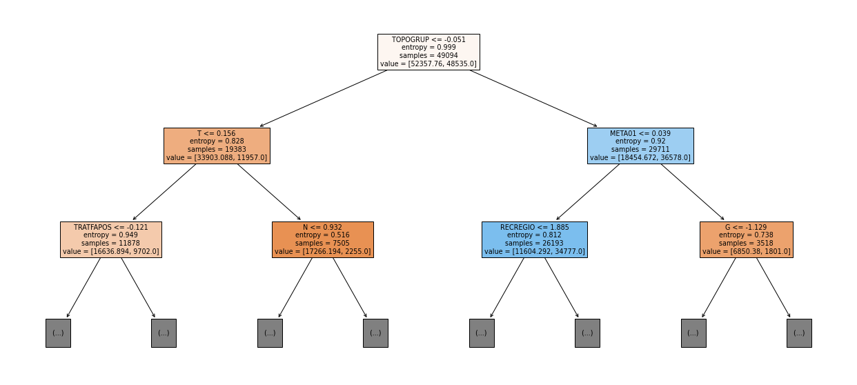
show_tree(rf_sp, feat_cols_SP, 2)
[ ]:
plot_roc_curve(rf_sp, X_train_SP, X_test_SP, y_train_SP, y_test_SP)
[ ]:
plot_feat_importances(rf_sp, feat_cols_SP)
The four most important features in the model were
ECGRUP,TOPO,TOPOGRUPandM.
[ ]:
plot_shap_values(rf_sp, X_test_SP, feat_cols_SP)
Note that larger values of the ECGRUP column, shown in pink, have more influence for the model’s prediction to be class 0, smaller values have greater weight for the prediction to be class 1. This behavior was expected, because the higher the clinical stage, worse is the stage of cancer.
The other columns shown follow the same logic.
[ ]:
# Other states
rf_fora = RandomForestClassifier(class_weight={0:1.75, 1:1},
                                 random_state=seed,
                                 criterion='entropy',
                                 max_depth=8)

rf_fora.fit(X_train_OS, y_train_OS)
RandomForestClassifier(class_weight={0: 1.75, 1: 1}, criterion='entropy',
                       max_depth=8, random_state=10)
[ ]:
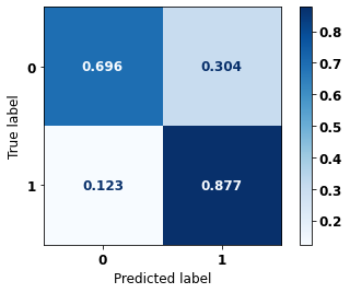
display_confusion_matrix(rf_fora, X_test_OS, y_test_OS)
              precision    recall  f1-score   support

           0      0.751     0.831     0.789      2413
           1      0.888     0.830     0.858      3907

    accuracy                          0.830      6320
   macro avg      0.820     0.830     0.824      6320
weighted avg      0.836     0.830     0.832      6320
The confusion matrix obtained for the Random Forest algorithm, with other states data, shows a good performance of the model, because the model achieves a 83% of accuracy.
[ ]:
show_tree(rf_fora, feat_cols_OS, 2)
[ ]:
plot_roc_curve(rf_fora, X_train_OS, X_test_OS, y_train_OS, y_test_OS)
[ ]:
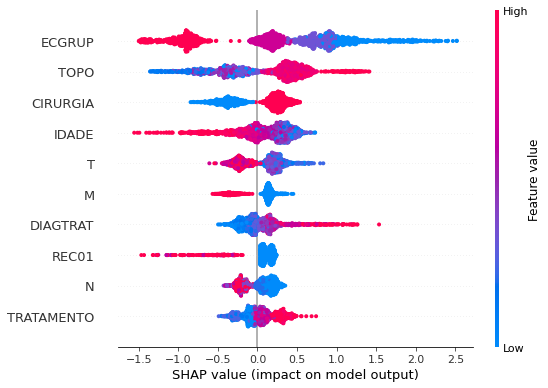
plot_feat_importances(rf_fora, feat_cols_OS)
The four most important features in the model were
ECGRUP,M,META01andTOPO.
[ ]:
plot_shap_values(rf_fora, X_test_OS, feat_cols_OS)
Note that larger values of the ECGRUP column, shown in pink, have more influence for the model’s prediction to be class 0, smaller values have greater weight for the prediction to be class 1. This behavior was expected, because the higher the clinical stage, worse is the stage of cancer.
The other columns shown follow the same logic.
XGBoost
The training of the XGBoost model follows the same pattern with random_state. A higher weight was also used for the class with fewer examples, using the hyperparameter scale_pos_weight.
The hyperparameter max_depth was chosen as 10 because the default value for this hyperparameter is 3, a low value for the amount of data we have.
[ ]:
# SP
xgboost_sp = XGBClassifier(max_depth=10,
                           scale_pos_weight=0.65,
                           random_state=seed)

xgboost_sp.fit(X_train_SP, y_train_SP)
XGBClassifier(max_depth=10, random_state=10, scale_pos_weight=0.65)
[ ]:
display_confusion_matrix(xgboost_sp, X_test_SP, y_test_SP)

              precision    recall  f1-score   support

           0      0.768     0.832     0.799     41022
           1      0.881     0.832     0.856     61274

    accuracy                          0.832    102296
   macro avg      0.825     0.832     0.827    102296
weighted avg      0.836     0.832     0.833    102296
The confusion matrix obtained for the XGBoost, with SP data, shows a good performance of the model, with 83% of accuracy.
[ ]:
plot_roc_curve(xgboost_sp, X_train_SP, X_test_SP, y_train_SP, y_test_SP)
[ ]:
plot_feat_importances(xgboost_sp, feat_cols_SP)
The four most important features in the model were
ECGRUP,HORMONIO,CIRURGIAandTOPO.
[ ]:
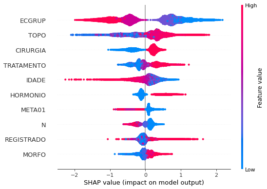
plot_shap_values(xgboost_sp, X_test_SP, feat_cols_SP)
Note that larger values of the ECGRUP column, shown in pink, have more influence for the model’s prediction to be class 0, smaller values have greater weight for the prediction to be class 1. This behavior was expected, because the higher the clinical stage, worse is the stage of cancer.
The other columns shown follow the same logic.
[ ]:
# Other states
xgboost_fora = XGBClassifier(max_depth=8,
                             scale_pos_weight=0.56,
                             random_state=seed)

xgboost_fora.fit(X_train_OS, y_train_OS)
XGBClassifier(max_depth=8, random_state=10, scale_pos_weight=0.56)
[ ]:
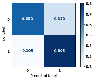
display_confusion_matrix(xgboost_fora, X_test_OS, y_test_OS)

              precision    recall  f1-score   support

           0      0.760     0.837     0.797      2413
           1      0.892     0.837     0.864      3907

    accuracy                          0.837      6320
   macro avg      0.826     0.837     0.830      6320
weighted avg      0.842     0.837     0.838      6320
The confusion matrix obtained for the XGBoost algorithm, with other states data, shows a good performance of the model, because the model achieves a 84% of accuracy.
[ ]:
plot_roc_curve(xgboost_fora, X_train_OS, X_test_OS, y_train_OS, y_test_OS)

[ ]:
plot_feat_importances(xgboost_fora, feat_cols_OS)
The four most important features in the model were
ECGRUP,CIRURGIA,HORMONIOandTOPO.
[ ]:
plot_shap_values(xgboost_fora, X_test_OS, feat_cols_OS)
Note that larger values of the ECGRUP column, shown in pink, have more influence for the model’s prediction to be class 0, smaller values have greater weight for the prediction to be class 1. This behavior was expected, because the higher the clinical stage, worse is the stage of cancer.
The other columns shown follow the same logic.
Third approach
Approach without columns EC and HORMONIO as features.
Preprocessing
Now we are going to divide the data into training and testing, and then do the preprocessing in both datasets to perform the training of the models and their evaluation.
First, it is necessary to define the columns that will be used as features and the label. We will not use some columns of the datasets: UFRESID, because we already have the division between SP and other states in the two datasets.
It was chosen to keep the column IDADE, so we will not use the FAIXAETAR, as well as the column ECGRUP and not the column EC. Finally, the other columns contained in the list list_drop are possible labels, so they will not be used as features for machine learning models.
[ ]:
list_drop = ['UFRESID', 'FAIXAETAR', 'ULTICONS', 'ULTIDIAG', 'ULTITRAT',
             'obito_geral', 'obito_cancer', 'vivo_ano1', 'vivo_ano5',
             'ULTINFO', 'EC', 'HORMONIO']

# 'RECNENHUM', 'RECLOCAL', 'RECREGIO', 'REC01', 'REC02', 'REC03', 'RECDIST'

lb = 'vivo_ano3'
A function was created to perform the preprocessing, preprocessing, that uses the other functions created, get_train_test (divides the dataset into train and test sets), train_preprocessing (do the preprocessing of the train set) and test_preprocessing (do the preprocessing of the test set).
To see the complete function go to the functions section.
SP
[ ]:
X_train_SP, X_test_SP, y_train_SP, y_test_SP, feat_cols_SP = preprocessing(df_SP_ano3, list_drop, lb,
                                                                           random_state=seed,
                                                                           balance_data=False,
                                                                           encoder_type='LabelEncoder',
                                                                           norm_name='StandardScaler')
X_train = (306886, 64), X_test = (102296, 64)
y_train = (306886,), y_test = (102296,)
Other states
[ ]:
X_train_OS, X_test_OS, y_train_OS, y_test_OS, feat_cols_OS = preprocessing(df_fora_ano3, list_drop, lb,
                                                                           random_state=seed,
                                                                           balance_data=False,
                                                                           encoder_type='LabelEncoder',
                                                                           norm_name='StandardScaler')
X_train = (18960, 64), X_test = (6320, 64)
y_train = (18960,), y_test = (6320,)
Training machine learning models
After dividing the data into training and testing, using the encoder and normalizing, the data is ready to be used by the machine learning models.
Random Forest
The first model that will be tested is the Random Forest, for this test the parameter random_state will be used, to obtain the same training values of the model every time it is runned.
The hyperparameter class_weight was also used, because the model has difficulty learning the class with fewer examples, so using this parameter this class will have a higher weight in the training of the model.
[ ]:
# SP
rf_sp = RandomForestClassifier(class_weight={0:1.56, 1:1},
                               random_state=seed,
                               criterion='entropy',
                               max_depth=10)

rf_sp.fit(X_train_SP, y_train_SP)
RandomForestClassifier(class_weight={0: 1.56, 1: 1}, criterion='entropy',
                       max_depth=10, random_state=10)
[ ]:
display_confusion_matrix(rf_sp, X_test_SP, y_test_SP)

              precision    recall  f1-score   support

           0      0.739     0.808     0.772     41022
           1      0.863     0.809     0.835     61274

    accuracy                          0.809    102296
   macro avg      0.801     0.809     0.804    102296
weighted avg      0.813     0.809     0.810    102296
The confusion matrix obtained for the Random Forest, with SP data, shows a good performance of the model, with 81% of accuracy.
[ ]:
show_tree(rf_sp, feat_cols_SP, 2)
[ ]:
plot_roc_curve(rf_sp, X_train_SP, X_test_SP, y_train_SP, y_test_SP)
[ ]:
plot_feat_importances(rf_sp, feat_cols_SP)
The four most important features in the model were
ECGRUP,TOPO,META01andTOPOGRUP.
[ ]:
plot_shap_values(rf_sp, X_test_SP, feat_cols_SP)
Note that larger values of the ECGRUP column, shown in pink, have more influence for the model’s prediction to be class 0, smaller values have greater weight for the prediction to be class 1. This behavior was expected, because the higher the clinical stage, worse is the stage of cancer.
The other columns shown follow the same logic.
[ ]:
# Other states
rf_fora = RandomForestClassifier(class_weight={0:1.747, 1:1},
                                 random_state=seed,
                                 criterion='entropy',
                                 max_depth=8)

rf_fora.fit(X_train_OS, y_train_OS)
RandomForestClassifier(class_weight={0: 1.747, 1: 1}, criterion='entropy',
                       max_depth=8, random_state=10)
[ ]:
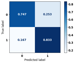
display_confusion_matrix(rf_fora, X_test_OS, y_test_OS)

              precision    recall  f1-score   support

           0      0.753     0.832     0.790      2413
           1      0.889     0.831     0.859      3907

    accuracy                          0.831      6320
   macro avg      0.821     0.832     0.825      6320
weighted avg      0.837     0.831     0.833      6320
The confusion matrix obtained for the Random Forest algorithm, with other states data, shows a good performance of the model, because the model achieves a 83% of accuracy.
[ ]:
show_tree(rf_fora, feat_cols_OS, 2)
[ ]:
plot_roc_curve(rf_fora, X_train_OS, X_test_OS, y_train_OS, y_test_OS)
[ ]:
plot_feat_importances(rf_fora, feat_cols_OS)
The four most important features in the model were
ECGRUP,META01,MandTOPO.
[ ]:
plot_shap_values(rf_fora, X_test_OS, feat_cols_OS)
Note that larger values of the ECGRUP column, shown in pink, have more influence for the model’s prediction to be class 0, smaller values have greater weight for the prediction to be class 1. This behavior was expected, because the higher the clinical stage, worse is the stage of cancer.
The other columns shown follow the same logic.
XGBoost
The training of the XGBoost model follows the same pattern with random_state. A higher weight was also used for the class with fewer examples, using the hyperparameter scale_pos_weight.
The hyperparameter max_depth was chosen as 10 because the default value for this hyperparameter is 3, a low value for the amount of data we have.
[ ]:
# SP
xgboost_sp = XGBClassifier(max_depth=10,
                           scale_pos_weight=0.64,
                           random_state=seed)

xgboost_sp.fit(X_train_SP, y_train_SP)
XGBClassifier(max_depth=10, random_state=10, scale_pos_weight=0.64)
[ ]:
display_confusion_matrix(xgboost_sp, X_test_SP, y_test_SP)

              precision    recall  f1-score   support

           0      0.767     0.832     0.798     41022
           1      0.881     0.831     0.855     61274

    accuracy                          0.831    102296
   macro avg      0.824     0.831     0.827    102296
weighted avg      0.835     0.831     0.832    102296
The confusion matrix obtained for the XGBoost, with SP data, shows a good performance of the model, with 83% of accuracy.
[ ]:
plot_roc_curve(xgboost_sp, X_train_SP, X_test_SP, y_train_SP, y_test_SP)

[ ]:
plot_feat_importances(xgboost_sp, feat_cols_SP)

The four most important features in the model were
ECGRUP,CIRURGIA,TRATAMENTOandTOPO.
[ ]:
plot_shap_values(xgboost_sp, X_test_SP, feat_cols_SP)
Note that larger values of the ECGRUP column, shown in pink, have more influence for the model’s prediction to be class 0, smaller values have greater weight for the prediction to be class 1. This behavior was expected, because the higher the clinical stage, worse is the stage of cancer.
The other columns shown follow the same logic.
[ ]:
# Other states
xgboost_fora = XGBClassifier(max_depth=8,
                             scale_pos_weight=0.555,
                             random_state=seed)

xgboost_fora.fit(X_train_OS, y_train_OS)
XGBClassifier(max_depth=8, random_state=10, scale_pos_weight=0.555)
[ ]:
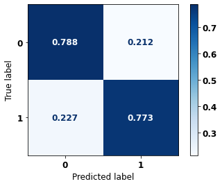
display_confusion_matrix(xgboost_fora, X_test_OS, y_test_OS)

              precision    recall  f1-score   support

           0      0.760     0.838     0.797      2413
           1      0.893     0.837     0.864      3907

    accuracy                          0.837      6320
   macro avg      0.827     0.837     0.831      6320
weighted avg      0.842     0.837     0.838      6320
The confusion matrix obtained for the XGBoost algorithm, with other states data, shows a good performance of the model, because the model achieves a 84% of accuracy.
[ ]:
plot_roc_curve(xgboost_fora, X_train_OS, X_test_OS, y_train_OS, y_test_OS)
[ ]:
plot_feat_importances(xgboost_fora, feat_cols_OS)
The four most important features in the model were
ECGRUP,CIRURGIA,TOPOandTRATAMENTO.
[ ]:
plot_shap_values(xgboost_fora, X_test_OS, feat_cols_OS)
Note that larger values of the ECGRUP column, shown in pink, have more influence for the model’s prediction to be class 0, smaller values have greater weight for the prediction to be class 1. This behavior was expected, because the higher the clinical stage, worse is the stage of cancer.
The other columns shown follow the same logic.
Fourth approach
Approach with grouped years and without the column EC.
Preprocessing
Now we are going to divide the data into training and testing, and then do the preprocessing in both datasets to perform the training of the models and their evaluation. We will use the years grouped too, resulting in 5 datasets for SP and more 5 for other states.
First, it is necessary to define the columns that will be used as features and the label. We will not use some columns of the datasets: UFRESID, because we already have the division between SP and other states in the two datasets.
It was chosen to keep the column IDADE, so we will not use the FAIXAETAR, as well as the column ECGRUP and not the column EC. Finally, the other columns contained in the list list_drop are possible labels, so they will not be used as features for machine learning models.
[ ]:
list_drop = ['UFRESID', 'FAIXAETAR', 'ULTICONS', 'ULTIDIAG', 'ULTITRAT',
             'obito_geral', 'obito_cancer', 'vivo_ano1', 'vivo_ano5', 'ULTINFO',
             'EC']

# 'RECNENHUM', 'RECLOCAL', 'RECREGIO', 'REC01', 'REC02', 'REC03', 'RECDIST'

lb = 'vivo_ano3'
A function was created to perform the preprocessing, preprocessing, that uses the other functions created, get_train_test (divides the dataset into train and test sets), train_preprocessing (do the preprocessing of the train set) and test_preprocessing (do the preprocessing of the test set).
The process will be done 5 times for SP and other states, using the datasets with grouped years.
To see the complete function go to the functions section.
SP
[ ]:
X_trainSP_00_03, X_testSP_00_03, y_trainSP_00_03, y_testSP_00_03, feat_SP_00_03 = preprocessing(df_SP_ano3, list_drop, lb,
                                                                                                group_years=True,
                                                                                                first_year=2000,
                                                                                                last_year=2003,
                                                                                                random_state=seed,
                                                                                                balance_data=False,
                                                                                                encoder_type='LabelEncoder',
                                                                                                norm_name='StandardScaler')
X_train = (45987, 65), X_test = (15329, 65)
y_train = (45987,), y_test = (15329,)
[ ]:
X_trainSP_04_07, X_testSP_04_07, y_trainSP_04_07, y_testSP_04_07, feat_SP_04_07 = preprocessing(df_SP_ano3, list_drop, lb,
                                                                                                group_years=True,
                                                                                                first_year=2004,
                                                                                                last_year=2007,
                                                                                                random_state=seed,
                                                                                                balance_data=False,
                                                                                                encoder_type='LabelEncoder',
                                                                                                norm_name='StandardScaler')
X_train = (57801, 65), X_test = (19267, 65)
y_train = (57801,), y_test = (19267,)
[ ]:
X_trainSP_08_11, X_testSP_08_11, y_trainSP_08_11, y_testSP_08_11, feat_SP_08_11 = preprocessing(df_SP_ano3, list_drop, lb,
                                                                                                group_years=True,
                                                                                                first_year=2008,
                                                                                                last_year=2011,
                                                                                                random_state=seed,
                                                                                                balance_data=False,
                                                                                                encoder_type='LabelEncoder',
                                                                                                norm_name='StandardScaler')
X_train = (77655, 65), X_test = (25886, 65)
y_train = (77655,), y_test = (25886,)
[ ]:
X_trainSP_12_15, X_testSP_12_15, y_trainSP_12_15, y_testSP_12_15, feat_SP_12_15 = preprocessing(df_SP_ano3, list_drop, lb,
                                                                                                group_years=True,
                                                                                                first_year=2012,
                                                                                                last_year=2015,
                                                                                                random_state=seed,
                                                                                                balance_data=False,
                                                                                                encoder_type='LabelEncoder',
                                                                                                norm_name='StandardScaler')
X_train = (89562, 65), X_test = (29854, 65)
y_train = (89562,), y_test = (29854,)
[ ]:
X_trainSP_16_21, X_testSP_16_21, y_trainSP_16_21, y_testSP_16_21, feat_SP_16_21 = preprocessing(df_SP_ano3, list_drop, lb,
                                                                                                group_years=True,
                                                                                                first_year=2016,
                                                                                                last_year=2021,
                                                                                                random_state=seed,
                                                                                                balance_data=False,
                                                                                                encoder_type='LabelEncoder',
                                                                                                norm_name='StandardScaler')
X_train = (35880, 65), X_test = (11961, 65)
y_train = (35880,), y_test = (11961,)
Other states
[ ]:
X_trainOS_00_03, X_testOS_00_03, y_trainOS_00_03, y_testOS_00_03, feat_OS_00_03 = preprocessing(df_fora_ano3, list_drop, lb,
                                                                                                group_years=True,
                                                                                                first_year=2000,
                                                                                                last_year=2003,
                                                                                                random_state=seed,
                                                                                                balance_data=False,
                                                                                                encoder_type='LabelEncoder',
                                                                                                norm_name='StandardScaler')
X_train = (2631, 65), X_test = (877, 65)
y_train = (2631,), y_test = (877,)
[ ]:
X_trainOS_04_07, X_testOS_04_07, y_trainOS_04_07, y_testOS_04_07, feat_OS_04_07 = preprocessing(df_fora_ano3, list_drop, lb,
                                                                                                group_years=True,
                                                                                                first_year=2004,
                                                                                                last_year=2007,
                                                                                                random_state=seed,
                                                                                                balance_data=False,
                                                                                                encoder_type='LabelEncoder',
                                                                                                norm_name='StandardScaler')
X_train = (3652, 65), X_test = (1218, 65)
y_train = (3652,), y_test = (1218,)
[ ]:
X_trainOS_08_11, X_testOS_08_11, y_trainOS_08_11, y_testOS_08_11, feat_OS_08_11 = preprocessing(df_fora_ano3, list_drop, lb,
                                                                                                group_years=True,
                                                                                                first_year=2008,
                                                                                                last_year=2011,
                                                                                                random_state=seed,
                                                                                                balance_data=False,
                                                                                                encoder_type='LabelEncoder',
                                                                                                norm_name='StandardScaler')
X_train = (4387, 65), X_test = (1463, 65)
y_train = (4387,), y_test = (1463,)
[ ]:
X_trainOS_12_15, X_testOS_12_15, y_trainOS_12_15, y_testOS_12_15, feat_OS_12_15 = preprocessing(df_fora_ano3, list_drop, lb,
                                                                                                group_years=True,
                                                                                                first_year=2012,
                                                                                                last_year=2015,
                                                                                                random_state=seed,
                                                                                                balance_data=False,
                                                                                                encoder_type='LabelEncoder',
                                                                                                norm_name='StandardScaler')
X_train = (5346, 65), X_test = (1782, 65)
y_train = (5346,), y_test = (1782,)
[ ]:
X_trainOS_16_20, X_testOS_16_20, y_trainOS_16_20, y_testOS_16_20, feat_OS_16_20 = preprocessing(df_fora_ano3, list_drop, lb,
                                                                                                group_years=True,
                                                                                                first_year=2016,
                                                                                                last_year=2020,
                                                                                                random_state=seed,
                                                                                                balance_data=False,
                                                                                                encoder_type='LabelEncoder',
                                                                                                norm_name='StandardScaler')
X_train = (2943, 65), X_test = (981, 65)
y_train = (2943,), y_test = (981,)
Training and evaluation of the models
After dividing the data into training and testing, using the encoder and normalizing, the data is ready to be used by the machine learning models.
Random Forest
The first model is the Random Forest, the random_state will be used as a parameter, to obtain the same training values of the model every time it is runned.
The hyperparameter class_weight was used because the models have difficulty to learn the class with fewer examples.
SP
[ ]:
# SP - 2000 to 2003
rf_sp_00_03 = RandomForestClassifier(random_state=seed,
                                     class_weight={0:1.4, 1:1},
                                     criterion='entropy',
                                     max_depth=10)

rf_sp_00_03.fit(X_trainSP_00_03, y_trainSP_00_03)
RandomForestClassifier(class_weight={0: 1.4, 1: 1}, criterion='entropy',
                       max_depth=10, random_state=10)
[ ]:
display_confusion_matrix(rf_sp_00_03, X_testSP_00_03, y_testSP_00_03)

              precision    recall  f1-score   support

           0      0.738     0.794     0.765      6483
           1      0.840     0.794     0.816      8846

    accuracy                          0.794     15329
   macro avg      0.789     0.794     0.791     15329
weighted avg      0.797     0.794     0.795     15329
The confusion matrix obtained for the Random Forest, with SP data from 2000 to 2003, shows a good performance of the model, with 79% of accuracy.
[ ]:
show_tree(rf_sp_00_03, feat_SP_00_03, 2)
[ ]:
plot_roc_curve(rf_sp_00_03, X_trainSP_00_03, X_testSP_00_03, y_trainSP_00_03, y_testSP_00_03)
[ ]:
plot_feat_importances(rf_sp_00_03, feat_SP_00_03)
The four most important features in the model were
ECGRUP,TOPO,TOPOGRUP, andM.
[ ]:
plot_shap_values(rf_sp_00_03, X_testSP_00_03, feat_SP_00_03)
Note that larger values of the ECGRUP column, shown in pink, have more influence for the model’s prediction to be class 0, smaller values have greater weight for the prediction to be class 1. This behavior was expected, because the higher the clinical stage, worse is the stage of cancer.
The other columns shown follow the same logic.
[ ]:
# SP - 2004 to 2007
rf_sp_04_07 = RandomForestClassifier(random_state=seed,
                                     class_weight={0:1.614, 1:1},
                                     criterion='entropy',
                                     max_depth=10)

rf_sp_04_07.fit(X_trainSP_04_07, y_trainSP_04_07)
RandomForestClassifier(class_weight={0: 1.614, 1: 1}, criterion='entropy',
                       max_depth=10, random_state=10)
[ ]:
display_confusion_matrix(rf_sp_04_07, X_testSP_04_07, y_testSP_04_07)

              precision    recall  f1-score   support

           0      0.722     0.800     0.759      7568
           1      0.861     0.801     0.830     11699

    accuracy                          0.801     19267
   macro avg      0.792     0.801     0.795     19267
weighted avg      0.807     0.801     0.802     19267
The confusion matrix obtained for the Random Forest, with SP data from 2004 to 2007, shows a good performance of the model, with 80% of accuracy.
[ ]:
show_tree(rf_sp_04_07, feat_SP_04_07, 2)
[ ]:
plot_roc_curve(rf_sp_04_07, X_trainSP_04_07, X_testSP_04_07, y_trainSP_04_07, y_testSP_04_07)

[ ]:
plot_feat_importances(rf_sp_04_07, feat_SP_04_07)
The four most important features in the model were
ECGRUP,TOPO,TOPOGRUPandM.
[ ]:
plot_shap_values(rf_sp_04_07, X_testSP_04_07, feat_SP_04_07)
Note that larger values of the ECGRUP column, shown in pink, have more influence for the model’s prediction to be class 0, smaller values have greater weight for the prediction to be class 1. This behavior was expected, because the higher the clinical stage, worse is the stage of cancer.
The other columns shown follow the same logic.
[ ]:
# SP - 2008 to 2011
rf_sp_08_11 = RandomForestClassifier(random_state=seed,
                                     class_weight={0:1.798, 1:1},
                                     criterion='entropy',
                                     max_depth=10)

rf_sp_08_11.fit(X_trainSP_08_11, y_trainSP_08_11)
RandomForestClassifier(class_weight={0: 1.798, 1: 1}, criterion='entropy',
                       max_depth=10, random_state=10)
[ ]:
display_confusion_matrix(rf_sp_08_11, X_testSP_08_11, y_testSP_08_11)

              precision    recall  f1-score   support

           0      0.719     0.812     0.763      9635
           1      0.879     0.812     0.844     16251

    accuracy                          0.812     25886
   macro avg      0.799     0.812     0.804     25886
weighted avg      0.820     0.812     0.814     25886
The confusion matrix obtained for the Random Forest, with SP data from 2008 to 2011, shows a good performance of the model, with 81% of accuracy.
[ ]:
show_tree(rf_sp_08_11, feat_SP_08_11, 2)
[ ]:
plot_roc_curve(rf_sp_08_11, X_trainSP_08_11, X_testSP_08_11, y_trainSP_08_11, y_testSP_08_11)
[ ]:
plot_feat_importances(rf_sp_08_11, feat_SP_08_11)
The four most important features in the model were
ECGRUP,TOPOGRUP,TOPOandM.
[ ]:
plot_shap_values(rf_sp_08_11, X_testSP_08_11, feat_SP_08_11)
Note that larger values of the ECGRUP column, shown in pink, have more influence for the model’s prediction to be class 0, smaller values have greater weight for the prediction to be class 1. This behavior was expected, because the higher the clinical stage, worse is the stage of cancer.
The other columns shown follow the same logic.
[ ]:
# SP - 2012 to 2015
rf_sp_12_15 = RandomForestClassifier(random_state=seed,
                                     class_weight={0:2, 1:1},
                                     criterion='entropy',
                                     max_depth=10)

rf_sp_12_15.fit(X_trainSP_12_15, y_trainSP_12_15)
RandomForestClassifier(class_weight={0: 2, 1: 1}, criterion='entropy',
                       max_depth=10, random_state=10)
[ ]:
display_confusion_matrix(rf_sp_12_15, X_testSP_12_15, y_testSP_12_15)

              precision    recall  f1-score   support

           0      0.702     0.811     0.753     10563
           1      0.887     0.812     0.848     19291

    accuracy                          0.812     29854
   macro avg      0.795     0.811     0.800     29854
weighted avg      0.822     0.812     0.814     29854
The confusion matrix obtained for the Random Forest, with SP data from 2012 to 2015, shows a good performance of the model with 81% of accuracy.
[ ]:
show_tree(rf_sp_12_15, feat_SP_12_15, 2)
[ ]:
plot_roc_curve(rf_sp_12_15, X_trainSP_12_15, X_testSP_12_15, y_trainSP_12_15, y_testSP_12_15)

[ ]:
plot_feat_importances(rf_sp_12_15, feat_SP_12_15)
The four most important features in the model were
ECGRUP,TOPO,MandTOPOGRUP.
[ ]:
plot_shap_values(rf_sp_12_15, X_testSP_12_15, feat_SP_12_15)
Note that larger values of the ECGRUP column, shown in pink, have more influence for the model’s prediction to be class 0, smaller values have greater weight for the prediction to be class 1. This behavior was expected, because the higher the clinical stage, worse is the stage of cancer.
The other columns shown follow the same logic.
[ ]:
# SP - 2016 to 2021
rf_sp_16_21 = RandomForestClassifier(random_state=seed,
                                     class_weight={0:1, 1:1.26},
                                     criterion='entropy',
                                     max_depth=10)

rf_sp_16_21.fit(X_trainSP_16_21, y_trainSP_16_21)
RandomForestClassifier(class_weight={0: 1, 1: 1.26}, criterion='entropy',
                       max_depth=10, random_state=10)
[ ]:
display_confusion_matrix(rf_sp_16_21, X_testSP_16_21, y_testSP_16_21)

              precision    recall  f1-score   support

           0      0.871     0.840     0.855      6773
           1      0.800     0.838     0.818      5188

    accuracy                          0.839     11961
   macro avg      0.835     0.839     0.837     11961
weighted avg      0.840     0.839     0.839     11961
The confusion matrix obtained for the Random Forest, with SP data from 2016 to 2021, shows a good performance of the model, with 84% of accuracy.
[ ]:
show_tree(rf_sp_16_21, feat_SP_16_21, 2)
[ ]:
plot_roc_curve(rf_sp_16_21, X_trainSP_16_21, X_testSP_16_21, y_trainSP_16_21, y_testSP_16_21)

[ ]:
plot_feat_importances(rf_sp_16_21, feat_SP_16_21)
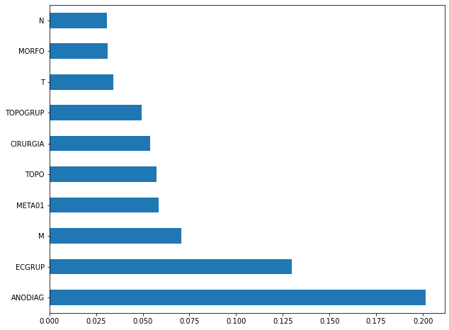
The four most important features in the model were
ANODIAG,ECGRUP,M, andMETA01.
[ ]:
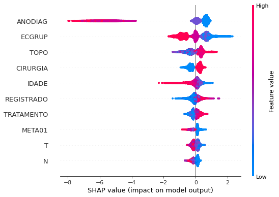
plot_shap_values(rf_sp_16_21, X_testSP_16_21, feat_SP_16_21)
Note that larger values of the ANODIAG column, shown in pink, have more influence for the model’s prediction to be class 0, smaller values have greater weight for the prediction to be class 1.
The other columns shown follow the same logic.
Other states
[ ]:
# Other states - 2000 to 2003
rf_fora_00_03 = RandomForestClassifier(random_state=seed,
                                       class_weight={0:1.776, 1:1},
                                       criterion='entropy',
                                       max_depth=6)

rf_fora_00_03.fit(X_trainOS_00_03, y_trainOS_00_03)
RandomForestClassifier(class_weight={0: 1.776, 1: 1}, criterion='entropy',
                       max_depth=6, random_state=10)
[ ]:
display_confusion_matrix(rf_fora_00_03, X_testOS_00_03, y_testOS_00_03)

              precision    recall  f1-score   support

           0      0.688     0.766     0.725       351
           1      0.831     0.768     0.798       526

    accuracy                          0.767       877
   macro avg      0.760     0.767     0.762       877
weighted avg      0.774     0.767     0.769       877
The confusion matrix obtained for the Random Forest, with other states data from 2000 to 2003, also shows a good performance of the model, and we have a balanced main diagonal with 77% of accuracy.
[ ]:
show_tree(rf_fora_00_03, feat_OS_00_03, 2)
[ ]:
plot_roc_curve(rf_fora_00_03, X_trainOS_00_03, X_testOS_00_03, y_trainOS_00_03, y_testOS_00_03)
[ ]:
plot_feat_importances(rf_fora_00_03, feat_OS_00_03)
The four most important features in the model were
ECGRUP,TOPO,TOPOGRUPandM.
[ ]:
plot_shap_values(rf_fora_00_03, X_testOS_00_03, feat_OS_00_03)
Note that larger values of the ECGRUP column, shown in pink, have more influence for the model’s prediction to be class 0, smaller values have greater weight for the prediction to be class 1. This behavior was expected, because the higher the clinical stage, worse is the stage of cancer.
The other columns shown follow the same logic.
[ ]:
# Other states - 2004 to 2007
rf_fora_04_07 = RandomForestClassifier(random_state=seed,
                                       class_weight={0:1.7, 1:1},
                                       criterion='entropy',
                                       max_depth=6)

rf_fora_04_07.fit(X_trainOS_04_07, y_trainOS_04_07)
RandomForestClassifier(class_weight={0: 1.7, 1: 1}, criterion='entropy',
                       max_depth=6, random_state=10)
[ ]:
display_confusion_matrix(rf_fora_04_07, X_testOS_04_07, y_testOS_04_07)
              precision    recall  f1-score   support

           0      0.701     0.804     0.749       443
           1      0.877     0.804     0.839       775

    accuracy                          0.804      1218
   macro avg      0.789     0.804     0.794      1218
weighted avg      0.813     0.804     0.806      1218
The confusion matrix obtained for the Random Forest, with other states data from 2004 to 2007, also shows a good performance of the model, with 80% of accuracy.
[ ]:
show_tree(rf_fora_04_07, feat_OS_04_07, 2)
[ ]:
plot_roc_curve(rf_fora_04_07, X_trainOS_04_07, X_testOS_04_07, y_trainOS_04_07, y_testOS_04_07)

[ ]:
plot_feat_importances(rf_fora_04_07, feat_OS_04_07)
The four most important features in the model were
ECGRUP,M,TandTOPO.
[ ]:
plot_shap_values(rf_fora_04_07, X_testOS_04_07, feat_OS_04_07)
Note that larger values of the ECGRUP column, shown in pink, have more influence for the model’s prediction to be class 0, smaller values have greater weight for the prediction to be class 1. This behavior was expected, because the higher the clinical stage, worse is the stage of cancer.
The other columns shown follow the same logic.
[ ]:
# Other states - 2008 to 2011
rf_fora_08_11 = RandomForestClassifier(random_state=seed,
                                       class_weight={0:2.31, 1:1},
                                       criterion='entropy',
                                       max_depth=6)

rf_fora_08_11.fit(X_trainOS_08_11, y_trainOS_08_11)
RandomForestClassifier(class_weight={0: 2.31, 1: 1}, criterion='entropy',
                       max_depth=6, random_state=10)
[ ]:
display_confusion_matrix(rf_fora_08_11, X_testOS_08_11, y_testOS_08_11)

              precision    recall  f1-score   support

           0      0.699     0.812     0.751       510
           1      0.890     0.813     0.850       953

    accuracy                          0.813      1463
   macro avg      0.795     0.812     0.801      1463
weighted avg      0.823     0.813     0.815      1463
The confusion matrix obtained for the Random Forest, with other states data from 2008 to 2011, also shows a good performance of the model, presenting 81% of accuracy.
[ ]:
show_tree(rf_fora_08_11, feat_OS_08_11, 2)

[ ]:
plot_roc_curve(rf_fora_08_11, X_trainOS_08_11, X_testOS_08_11, y_trainOS_08_11, y_testOS_08_11)
[ ]:
plot_feat_importances(rf_fora_08_11, feat_OS_08_11)
The four most important features in the model were
ECGRUP,M,NandMETA01.
[ ]:
plot_shap_values(rf_fora_08_11, X_testOS_08_11, feat_OS_08_11)
Note that larger values of the ECGRUP column, shown in pink, have more influence for the model’s prediction to be class 0, smaller values have greater weight for the prediction to be class 1. This behavior was expected, because the higher the clinical stage, worse is the stage of cancer.
The other columns shown follow the same logic.
[ ]:
# Other states - 2012 to 2015
rf_fora_12_15 = RandomForestClassifier(random_state=seed,
                                       class_weight={0:2.9, 1:1},
                                       criterion='entropy',
                                       max_depth=7)

rf_fora_12_15.fit(X_trainOS_12_15, y_trainOS_12_15)
RandomForestClassifier(class_weight={0: 2.9, 1: 1}, criterion='entropy',
                       max_depth=7, random_state=10)
[ ]:
display_confusion_matrix(rf_fora_12_15, X_testOS_12_15, y_testOS_12_15)

              precision    recall  f1-score   support

           0      0.670     0.813     0.734       571
           1      0.902     0.811     0.854      1211

    accuracy                          0.811      1782
   macro avg      0.786     0.812     0.794      1782
weighted avg      0.827     0.811     0.816      1782
The confusion matrix obtained for the Random Forest, with other states data from 2012 to 2015, also shows a good performance of the model, presenting 81% of accuracy.
[ ]:
show_tree(rf_fora_12_15, feat_OS_12_15, 2)
[ ]:
plot_roc_curve(rf_fora_12_15, X_trainOS_12_15, X_testOS_12_15, y_trainOS_12_15, y_testOS_12_15)
[ ]:
plot_feat_importances(rf_fora_12_15, feat_OS_12_15)
The four most important features in the model were
ECGRUP,M,TOPOandTOPOGRUP.
[ ]:
plot_shap_values(rf_fora_12_15, X_testOS_12_15, feat_OS_12_15)
Note that larger values of the ECGRUP column, shown in pink, have more influence for the model’s prediction to be class 0, smaller values have greater weight for the prediction to be class 1. This behavior was expected, because the higher the clinical stage, worse is the stage of cancer.
The other columns shown follow the same logic.
[ ]:
# Other states - 2016 to 2020
rf_fora_16_20 = RandomForestClassifier(random_state=seed,
                                       class_weight={0:1, 1:1},
                                       criterion='entropy',
                                       max_depth=8)

rf_fora_16_20.fit(X_trainOS_16_20, y_trainOS_16_20)
RandomForestClassifier(class_weight={0: 1, 1: 1}, criterion='entropy',
                       max_depth=8, random_state=10)
[ ]:
display_confusion_matrix(rf_fora_16_20, X_testOS_16_20, y_testOS_16_20)
              precision    recall  f1-score   support

           0      0.870     0.848     0.859       539
           1      0.820     0.846     0.833       442

    accuracy                          0.847       981
   macro avg      0.845     0.847     0.846       981
weighted avg      0.848     0.847     0.847       981
The confusion matrix obtained for the Random Forest, with other states data from 2016 to 2020, also shows a good performance of the model, presenting 85% of accuracy.
[ ]:
show_tree(rf_fora_16_20, feat_OS_16_20, 2)
[ ]:
plot_roc_curve(rf_fora_16_20, X_trainOS_16_20, X_testOS_16_20, y_trainOS_16_20, y_testOS_16_20)
[ ]:
plot_feat_importances(rf_fora_16_20, feat_OS_16_20)
The four most important features in the model were
ANODIAG,ECGRUP,MandCIRURGIA.
[ ]:
plot_shap_values(rf_fora_16_20, X_testOS_16_20, feat_OS_16_20)
Note that larger values of the ANODIAG column, shown in pink, have more influence for the model’s prediction to be class 0, smaller values have greater weight for the prediction to be class 1.
The other columns shown follow the same logic.
XGBoost
The training of the XGBoost models follows the same pattern with random_state. The hyperparameter scale_pos_weight was also used in some trainings, in order to obtain a balanced main diagonal in the confusion matrix.
The hyperparameter max_depth was chosen as 10 because the default value for this hyperparameter is 3, a low value for the amount of data we have.
SP
[ ]:
# SP - 2000 to 2003
xgb_sp_00_03 = XGBClassifier(max_depth=8,
                             random_state=seed,
                             scale_pos_weight=0.71)

xgb_sp_00_03.fit(X_trainSP_00_03, y_trainSP_00_03)
XGBClassifier(max_depth=8, random_state=10, scale_pos_weight=0.71)
[ ]:
display_confusion_matrix(xgb_sp_00_03, X_testSP_00_03, y_testSP_00_03)
              precision    recall  f1-score   support

           0      0.758     0.812     0.784      6483
           1      0.855     0.810     0.832      8846

    accuracy                          0.811     15329
   macro avg      0.806     0.811     0.808     15329
weighted avg      0.814     0.811     0.812     15329
The confusion matrix obtained for the XGBoost, with SP data from 2000 to 2003, shows a good performance of the model, here with 81% of accuracy.
[ ]:
plot_roc_curve(xgb_sp_00_03, X_trainSP_00_03, X_testSP_00_03, y_trainSP_00_03, y_testSP_00_03)
[ ]:
plot_feat_importances(xgb_sp_00_03, feat_SP_00_03)
The four most important features in the model were
ECGRUP,HORMONIO,MandCIRURGIA.
[ ]:
plot_shap_values(xgb_sp_00_03, X_testSP_00_03, feat_SP_00_03)
Note that larger values of the ECGRUP column, shown in pink, have more influence for the model’s prediction to be class 0, smaller values have greater weight for the prediction to be class 1. This behavior was expected, because the higher the clinical stage, worse is the stage of cancer.
The other columns shown follow the same logic.
[ ]:
# SP - 2004 to 2007
xgb_sp_04_07 = XGBClassifier(max_depth=8,
                             random_state=seed,
                             scale_pos_weight=0.635)

xgb_sp_04_07.fit(X_trainSP_04_07, y_trainSP_04_07)
XGBClassifier(max_depth=8, random_state=10, scale_pos_weight=0.635)
[ ]:
display_confusion_matrix(xgb_sp_04_07, X_testSP_04_07, y_testSP_04_07)
              precision    recall  f1-score   support

           0      0.746     0.821     0.782      7568
           1      0.876     0.820     0.847     11699

    accuracy                          0.820     19267
   macro avg      0.811     0.820     0.814     19267
weighted avg      0.825     0.820     0.821     19267
The confusion matrix obtained for the XGBoost, with SP data from 2004 to 2007, shows a good performance of the model, with 82% of accuracy.
[ ]:
plot_roc_curve(xgb_sp_04_07, X_trainSP_04_07, X_testSP_04_07, y_trainSP_04_07, y_testSP_04_07)

[ ]:
plot_feat_importances(xgb_sp_04_07, feat_SP_04_07)
Here we noticed that the most used feature was
ECGRUP, with some advantage over the others. Following we haveHORMONIO,CIRURGIAandMETA01.
[ ]:
plot_shap_values(xgb_sp_04_07, X_testSP_04_07, feat_SP_04_07)
Note that larger values of the ECGRUP column, shown in pink, have more influence for the model’s prediction to be class 0, smaller values have greater weight for the prediction to be class 1. This behavior was expected, because the higher the clinical stage, worse is the stage of cancer.
The other columns shown follow the same logic.
[ ]:
# SP - 2008 to 2011
xgb_sp_08_11 = XGBClassifier(max_depth=8,
                             scale_pos_weight=0.5605,
                             random_state=seed)

xgb_sp_08_11.fit(X_trainSP_08_11, y_trainSP_08_11)
XGBClassifier(max_depth=8, random_state=10, scale_pos_weight=0.5605)
[ ]:
display_confusion_matrix(xgb_sp_08_11, X_testSP_08_11, y_testSP_08_11)

              precision    recall  f1-score   support

           0      0.738     0.825     0.779      9635
           1      0.889     0.826     0.856     16251

    accuracy                          0.826     25886
   macro avg      0.813     0.826     0.818     25886
weighted avg      0.832     0.826     0.827     25886
The confusion matrix obtained for the XGBoost, with SP data from 2008 to 2011, shows a good performance of the model, with 83% of accuracy.
[ ]:
plot_roc_curve(xgb_sp_08_11, X_trainSP_08_11, X_testSP_08_11, y_trainSP_08_11, y_testSP_08_11)

[ ]:
plot_feat_importances(xgb_sp_08_11, feat_SP_08_11)
Here we noticed that the most used feature was
ECGRUP, with a good advantage over the others. Following we haveHORMONIO,CIRURGIAandMETA01.
[ ]:
plot_shap_values(xgb_sp_08_11, X_testSP_08_11, feat_SP_08_11)
Note that larger values of the ECGRUP column, shown in pink, have more influence for the model’s prediction to be class 0, smaller values have greater weight for the prediction to be class 1. This behavior was expected, because the higher the clinical stage, worse is the stage of cancer.
The other columns shown follow the same logic.
[ ]:
# SP - 2012 to 2015
xgb_sp_12_15 = XGBClassifier(max_depth=8,
                             random_state=seed,
                             scale_pos_weight=0.51)

xgb_sp_12_15.fit(X_trainSP_12_15, y_trainSP_12_15)
XGBClassifier(max_depth=8, random_state=10, scale_pos_weight=0.51)
[ ]:
display_confusion_matrix(xgb_sp_12_15, X_testSP_12_15, y_testSP_12_15)

              precision    recall  f1-score   support

           0      0.720     0.825     0.769     10563
           1      0.896     0.824     0.858     19291

    accuracy                          0.824     29854
   macro avg      0.808     0.825     0.814     29854
weighted avg      0.834     0.824     0.827     29854
The confusion matrix obtained for the XGBoost, with SP data from 2012 to 2015, shows a good performance of the model, with 82% of accuracy.
[ ]:
plot_roc_curve(xgb_sp_12_15, X_trainSP_12_15, X_testSP_12_15, y_trainSP_12_15, y_testSP_12_15)
[ ]:
plot_feat_importances(xgb_sp_12_15, feat_SP_12_15)
Here we noticed that the most used feature was
ECGRUP, with a good advantage. Following we haveCIRURGIA,HORMONIOandTOPO.
[ ]:
plot_shap_values(xgb_sp_12_15, X_testSP_12_15, feat_SP_12_15)
Note that larger values of the ECGRUP column, shown in pink, have more influence for the model’s prediction to be class 0, smaller values have greater weight for the prediction to be class 1. This behavior was expected, because the higher the clinical stage, worse is the stage of cancer.
The other columns shown follow the same logic.
[ ]:
# SP - 2016 to 2021
xgb_sp_16_21 = XGBClassifier(max_depth=8,
                             random_state=seed,
                             scale_pos_weight=1.26)

xgb_sp_16_21.fit(X_trainSP_16_21, y_trainSP_16_21)
XGBClassifier(max_depth=8, random_state=10, scale_pos_weight=1.26)
[ ]:
display_confusion_matrix(xgb_sp_16_21, X_testSP_16_21, y_testSP_16_21)

              precision    recall  f1-score   support

           0      0.888     0.858     0.872      6773
           1      0.822     0.858     0.840      5188

    accuracy                          0.858     11961
   macro avg      0.855     0.858     0.856     11961
weighted avg      0.859     0.858     0.858     11961
The confusion matrix obtained for the XGBoost, with SP data from 2016 to 2021, shows a good performance of the model, with 86% of accuracy.
[ ]:
plot_roc_curve(xgb_sp_16_21, X_trainSP_16_21, X_testSP_16_21, y_trainSP_16_21, y_testSP_16_21)
[ ]:
plot_feat_importances(xgb_sp_16_21, feat_SP_16_21)
The four most important features were
ECGRUP,ANODIAG,RECDISTandHORMONIO.
[ ]:
plot_shap_values(xgb_sp_16_21, X_testSP_16_21, feat_SP_16_21)
Note that larger values of the ANODIAG column, shown in pink, have more influence for the model’s prediction to be class 0, smaller values have greater weight for the prediction to be class 1.
The other columns shown follow the same logic.
Other states
[ ]:
# Other states - 2000 to 2003
xgb_fora_00_03 = XGBClassifier(max_depth=4,
                               scale_pos_weight=0.55,
                               random_state=seed)

xgb_fora_00_03.fit(X_trainOS_00_03, y_trainOS_00_03)
XGBClassifier(max_depth=4, random_state=10, scale_pos_weight=0.55)
[ ]:
display_confusion_matrix(xgb_fora_00_03, X_testOS_00_03, y_testOS_00_03)
              precision    recall  f1-score   support

           0      0.700     0.778     0.737       351
           1      0.840     0.778     0.808       526

    accuracy                          0.778       877
   macro avg      0.770     0.778     0.772       877
weighted avg      0.784     0.778     0.779       877
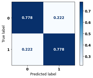
The confusion matrix obtained for the XGBoost, with other states data from 2000 to 2003, also shows a good performance of the model, with 78% of accuracy.
[ ]:
plot_roc_curve(xgb_fora_00_03, X_trainOS_00_03, X_testOS_00_03, y_trainOS_00_03, y_testOS_00_03)

[ ]:
plot_feat_importances(xgb_fora_00_03, feat_OS_00_03)
The four most important features in the model were
ECGRUP,HORMONIO,RECLOCALandTOPO.
[ ]:
plot_shap_values(xgb_fora_00_03, X_testOS_00_03, feat_OS_00_03)
Note that larger values of the ECGRUP column, shown in pink, have more influence for the model’s prediction to be class 0, smaller values have greater weight for the prediction to be class 1. This behavior was expected, because the higher the clinical stage, worse is the stage of cancer.
The other columns shown follow the same logic.
[ ]:
# Other states - 2004 to 2007
xgb_fora_04_07 = XGBClassifier(max_depth=4,
                               scale_pos_weight=0.6,
                               random_state=seed)

xgb_fora_04_07.fit(X_trainOS_04_07, y_trainOS_04_07)
XGBClassifier(max_depth=4, random_state=10, scale_pos_weight=0.6)
[ ]:
display_confusion_matrix(xgb_fora_04_07, X_testOS_04_07, y_testOS_04_07)

              precision    recall  f1-score   support

           0      0.709     0.810     0.757       443
           1      0.882     0.810     0.845       775

    accuracy                          0.810      1218
   macro avg      0.796     0.810     0.801      1218
weighted avg      0.819     0.810     0.813      1218
The confusion matrix obtained for the XGBoost, with other states data from 2004 to 2007, also shows a good performance of the model with 81% of accuracy.
[ ]:
plot_roc_curve(xgb_fora_04_07, X_trainOS_04_07, X_testOS_04_07, y_trainOS_04_07, y_testOS_04_07)
[ ]:
plot_feat_importances(xgb_fora_04_07, feat_OS_04_07)
Again we noticed that the most used feature was
ECGRUP, with a good advantage. The following most important features wereMETA01,TandMORFO.
[ ]:
plot_shap_values(xgb_fora_04_07, X_testOS_04_07, feat_OS_04_07)
Note that larger values of the ECGRUP column, shown in pink, have more influence for the model’s prediction to be class 0, smaller values have greater weight for the prediction to be class 1. This behavior was expected, because the higher the clinical stage, worse is the stage of cancer.
The other columns shown follow the same logic.
[ ]:
# Other states - 2008 to 2011
xgb_fora_08_11 = XGBClassifier(max_depth=4,
                               scale_pos_weight=0.49,
                               random_state=seed)

xgb_fora_08_11.fit(X_trainOS_08_11, y_trainOS_08_11)
XGBClassifier(max_depth=4, random_state=10, scale_pos_weight=0.49)
[ ]:
display_confusion_matrix(xgb_fora_08_11, X_testOS_08_11, y_testOS_08_11)

              precision    recall  f1-score   support

           0      0.716     0.825     0.767       510
           1      0.898     0.825     0.860       953

    accuracy                          0.825      1463
   macro avg      0.807     0.825     0.813      1463
weighted avg      0.835     0.825     0.827      1463
The confusion matrix obtained for the XGBoost, with other states data from 2008 to 2011, also shows a good performance of the model with 82% of accuracy.
[ ]:
plot_roc_curve(xgb_fora_08_11, X_trainOS_08_11, X_testOS_08_11, y_trainOS_08_11, y_testOS_08_11)
[ ]:
plot_feat_importances(xgb_fora_08_11, feat_OS_08_11)
Again we noticed that the most used feature was
ECGRUP, with a lot advantage. The following most important features wereM,HORMONIOandCIRURGIA.
[ ]:
plot_shap_values(xgb_fora_08_11, X_testOS_08_11, feat_OS_08_11)
Note that larger values of the ECGRUP column, shown in pink, have more influence for the model’s prediction to be class 0, smaller values have greater weight for the prediction to be class 1. This behavior was expected, because the higher the clinical stage, worse is the stage of cancer.
The other columns shown follow the same logic.
[ ]:
# Other states - 2012 to 2015
xgb_fora_12_15 = XGBClassifier(max_depth=5,
                               scale_pos_weight=0.37,
                               random_state=seed)

xgb_fora_12_15.fit(X_trainOS_12_15, y_trainOS_12_15)
XGBClassifier(max_depth=5, random_state=10, scale_pos_weight=0.37)
[ ]:
display_confusion_matrix(xgb_fora_12_15, X_testOS_12_15, y_testOS_12_15)

              precision    recall  f1-score   support

           0      0.687     0.823     0.749       571
           1      0.908     0.823     0.864      1211

    accuracy                          0.823      1782
   macro avg      0.798     0.823     0.806      1782
weighted avg      0.837     0.823     0.827      1782
The confusion matrix obtained for the XGBoost, with other states data from 2012 to 2015, also shows a good performance of the model with 82% of accuracy.
[ ]:
plot_roc_curve(xgb_fora_12_15, X_trainOS_12_15, X_testOS_12_15, y_trainOS_12_15, y_testOS_12_15)
[ ]:
plot_feat_importances(xgb_fora_12_15, feat_OS_12_15)
The four most important features were
ECGRUP,M,CIRURGIAandREC01.
[ ]:
plot_shap_values(xgb_fora_12_15, X_testOS_12_15, feat_OS_12_15)
Note that larger values of the ECGRUP column, shown in pink, have more influence for the model’s prediction to be class 0, smaller values have greater weight for the prediction to be class 1. This behavior was expected, because the higher the clinical stage, worse is the stage of cancer.
The other columns shown follow the same logic.
[ ]:
# Other states - 2016 to 2020
xgb_fora_16_20 = XGBClassifier(max_depth=5,
                               scale_pos_weight=1.04,
                               random_state=seed)

xgb_fora_16_20.fit(X_trainOS_16_20, y_trainOS_16_20)
XGBClassifier(max_depth=5, random_state=10, scale_pos_weight=1.04)
[ ]:
display_confusion_matrix(xgb_fora_16_20, X_testOS_16_20, y_testOS_16_20)

              precision    recall  f1-score   support

           0      0.880     0.855     0.867       539
           1      0.829     0.857     0.843       442

    accuracy                          0.856       981
   macro avg      0.855     0.856     0.855       981
weighted avg      0.857     0.856     0.856       981
The confusion matrix obtained for the XGBoost, with other states data from 2016 to 2020, shows the best performance comparing with the other models, with 86% of accuracy.
[ ]:
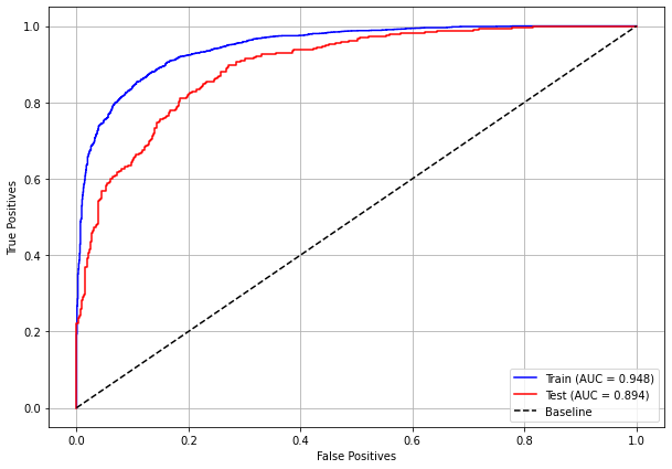
plot_roc_curve(xgb_fora_16_20, X_trainOS_16_20, X_testOS_16_20, y_trainOS_16_20, y_testOS_16_20)
[ ]:
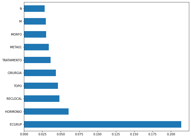
plot_feat_importances(xgb_fora_16_20, feat_OS_16_20)
The four most important features were
ECGRUP,META01,ANODIAGandRECDIST.
[ ]:
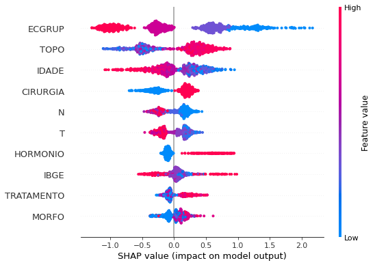
plot_shap_values(xgb_fora_16_20, X_testOS_16_20, feat_OS_16_20)
Note that larger values of the ANODIAG column, shown in pink, have more influence for the model’s prediction to be class 0, smaller values have greater weight for the prediction to be class 1.
The other columns shown follow the same logic.
Testing models with data from other years
We will use test data from the following years in the trained models for each set of years grouped together.
Random Forest SP for years 2000 to 2003
[ ]:
display_confusion_matrix(rf_sp_00_03, X_testSP_04_07, y_testSP_04_07)
              precision    recall  f1-score   support

           0      0.726     0.790     0.757      7568
           1      0.856     0.807     0.831     11699

    accuracy                          0.801     19267
   macro avg      0.791     0.799     0.794     19267
weighted avg      0.805     0.801     0.802     19267
[ ]:
display_confusion_matrix(rf_sp_00_03, X_testSP_08_11, y_testSP_08_11)
              precision    recall  f1-score   support

           0      0.710     0.779     0.743      9635
           1      0.861     0.812     0.836     16251

    accuracy                          0.799     25886
   macro avg      0.786     0.795     0.789     25886
weighted avg      0.805     0.799     0.801     25886
[ ]:
display_confusion_matrix(rf_sp_00_03, X_testSP_12_15, y_testSP_12_15)
              precision    recall  f1-score   support

           0      0.684     0.788     0.732     10563
           1      0.873     0.801     0.835     19291

    accuracy                          0.796     29854
   macro avg      0.779     0.794     0.784     29854
weighted avg      0.806     0.796     0.799     29854
[ ]:
display_confusion_matrix(rf_sp_00_03, X_testSP_16_21, y_testSP_16_21)

              precision    recall  f1-score   support

           0      0.826     0.791     0.808      6773
           1      0.742     0.782     0.761      5188

    accuracy                          0.787     11961
   macro avg      0.784     0.787     0.785     11961
weighted avg      0.789     0.787     0.788     11961
XGBoost SP for years 2000 to 2003
[ ]:
display_confusion_matrix(xgb_sp_00_03, X_testSP_04_07, y_testSP_04_07)

              precision    recall  f1-score   support

           0      0.757     0.763     0.760      7568
           1      0.846     0.842     0.844     11699

    accuracy                          0.811     19267
   macro avg      0.802     0.802     0.802     19267
weighted avg      0.811     0.811     0.811     19267
[ ]:
display_confusion_matrix(xgb_sp_00_03, X_testSP_08_11, y_testSP_08_11)

              precision    recall  f1-score   support

           0      0.742     0.740     0.741      9635
           1      0.846     0.848     0.847     16251

    accuracy                          0.807     25886
   macro avg      0.794     0.794     0.794     25886
weighted avg      0.807     0.807     0.807     25886
[ ]:
display_confusion_matrix(xgb_sp_00_03, X_testSP_12_15, y_testSP_12_15)

              precision    recall  f1-score   support

           0      0.718     0.726     0.722     10563
           1      0.849     0.844     0.846     19291

    accuracy                          0.802     29854
   macro avg      0.783     0.785     0.784     29854
weighted avg      0.803     0.802     0.802     29854
[ ]:
display_confusion_matrix(xgb_sp_00_03, X_testSP_16_21, y_testSP_16_21)
              precision    recall  f1-score   support

           0      0.829     0.743     0.784      6773
           1      0.705     0.800     0.749      5188

    accuracy                          0.768     11961
   macro avg      0.767     0.772     0.767     11961
weighted avg      0.775     0.768     0.769     11961
Random Forest SP for years 2004 to 2007
[ ]:
display_confusion_matrix(rf_sp_04_07, X_testSP_08_11, y_testSP_08_11)
              precision    recall  f1-score   support

           0      0.702     0.797     0.746      9635
           1      0.869     0.800     0.833     16251

    accuracy                          0.799     25886
   macro avg      0.786     0.798     0.790     25886
weighted avg      0.807     0.799     0.801     25886
[ ]:
display_confusion_matrix(rf_sp_04_07, X_testSP_12_15, y_testSP_12_15)

              precision    recall  f1-score   support

           0      0.679     0.796     0.733     10563
           1      0.877     0.794     0.833     19291

    accuracy                          0.795     29854
   macro avg      0.778     0.795     0.783     29854
weighted avg      0.807     0.795     0.798     29854
[ ]:
display_confusion_matrix(rf_sp_04_07, X_testSP_16_21, y_testSP_16_21)

              precision    recall  f1-score   support

           0      0.827     0.791     0.809      6773
           1      0.742     0.784     0.762      5188

    accuracy                          0.788     11961
   macro avg      0.784     0.787     0.785     11961
weighted avg      0.790     0.788     0.789     11961
XGBoost SP for years 2004 to 2007
[ ]:
display_confusion_matrix(xgb_sp_04_07, X_testSP_08_11, y_testSP_08_11)

              precision    recall  f1-score   support

           0      0.736     0.775     0.755      9635
           1      0.862     0.836     0.849     16251

    accuracy                          0.813     25886
   macro avg      0.799     0.805     0.802     25886
weighted avg      0.815     0.813     0.814     25886
[ ]:
display_confusion_matrix(xgb_sp_04_07, X_testSP_12_15, y_testSP_12_15)
              precision    recall  f1-score   support

           0      0.710     0.747     0.728     10563
           1      0.857     0.833     0.845     19291

    accuracy                          0.802     29854
   macro avg      0.783     0.790     0.786     29854
weighted avg      0.805     0.802     0.803     29854
[ ]:
display_confusion_matrix(xgb_sp_04_07, X_testSP_16_21, y_testSP_16_21)

              precision    recall  f1-score   support

           0      0.839     0.713     0.771      6773
           1      0.687     0.822     0.748      5188

    accuracy                          0.760     11961
   macro avg      0.763     0.768     0.760     11961
weighted avg      0.773     0.760     0.761     11961
Random Forest SP for years 2008 to 2011
[ ]:
display_confusion_matrix(rf_sp_08_11, X_testSP_12_15, y_testSP_12_15)

              precision    recall  f1-score   support

           0      0.711     0.772     0.740     10563
           1      0.869     0.828     0.848     19291

    accuracy                          0.808     29854
   macro avg      0.790     0.800     0.794     29854
weighted avg      0.813     0.808     0.810     29854
[ ]:
display_confusion_matrix(rf_sp_08_11, X_testSP_16_21, y_testSP_16_21)
              precision    recall  f1-score   support

           0      0.819     0.788     0.803      6773
           1      0.736     0.773     0.754      5188

    accuracy                          0.781     11961
   macro avg      0.777     0.780     0.778     11961
weighted avg      0.783     0.781     0.782     11961
XGBoost SP for years 2008 to 2011
[ ]:
display_confusion_matrix(xgb_sp_08_11, X_testSP_12_15, y_testSP_12_15)
              precision    recall  f1-score   support

           0      0.756     0.696     0.725     10563
           1      0.840     0.877     0.858     19291

    accuracy                          0.813     29854
   macro avg      0.798     0.786     0.791     29854
weighted avg      0.810     0.813     0.811     29854
[ ]:
display_confusion_matrix(xgb_sp_08_11, X_testSP_16_21, y_testSP_16_21)
              precision    recall  f1-score   support

           0      0.822     0.690     0.750      6773
           1      0.665     0.805     0.728      5188

    accuracy                          0.740     11961
   macro avg      0.743     0.747     0.739     11961
weighted avg      0.754     0.740     0.741     11961
Random Forest SP for years 2012 to 2015
[ ]:
display_confusion_matrix(rf_sp_12_15, X_testSP_16_21, y_testSP_16_21)

              precision    recall  f1-score   support

           0      0.825     0.817     0.821      6773
           1      0.764     0.774     0.769      5188

    accuracy                          0.798     11961
   macro avg      0.794     0.795     0.795     11961
weighted avg      0.798     0.798     0.798     11961
XGBoost SP for years 2012 to 2015
[ ]:
display_confusion_matrix(xgb_sp_12_15, X_testSP_16_21, y_testSP_16_21)

              precision    recall  f1-score   support

           0      0.814     0.827     0.820      6773
           1      0.769     0.754     0.761      5188

    accuracy                          0.795     11961
   macro avg      0.792     0.790     0.791     11961
weighted avg      0.795     0.795     0.795     11961
Random Forest Other states for years 2000 to 2003
[ ]:
display_confusion_matrix(rf_fora_00_03, X_testOS_04_07, y_testOS_04_07)

              precision    recall  f1-score   support

           0      0.670     0.815     0.735       443
           1      0.879     0.770     0.821       775

    accuracy                          0.787      1218
   macro avg      0.774     0.793     0.778      1218
weighted avg      0.803     0.787     0.790      1218
[ ]:
display_confusion_matrix(rf_fora_00_03, X_testOS_08_11, y_testOS_08_11)

              precision    recall  f1-score   support

           0      0.656     0.865     0.746       510
           1      0.913     0.758     0.828       953

    accuracy                          0.795      1463
   macro avg      0.785     0.811     0.787      1463
weighted avg      0.823     0.795     0.799      1463
[ ]:
display_confusion_matrix(rf_fora_00_03, X_testOS_12_15, y_testOS_12_15)

              precision    recall  f1-score   support

           0      0.619     0.842     0.714       571
           1      0.910     0.756     0.826      1211

    accuracy                          0.783      1782
   macro avg      0.765     0.799     0.770      1782
weighted avg      0.817     0.783     0.790      1782
[ ]:
display_confusion_matrix(rf_fora_00_03, X_testOS_16_20, y_testOS_16_20)

              precision    recall  f1-score   support

           0      0.808     0.842     0.825       539
           1      0.797     0.756     0.776       442

    accuracy                          0.803       981
   macro avg      0.802     0.799     0.800       981
weighted avg      0.803     0.803     0.803       981
XGBoost Other states for years 2000 to 2003
[ ]:
display_confusion_matrix(xgb_fora_00_03, X_testOS_04_07, y_testOS_04_07)

              precision    recall  f1-score   support

           0      0.670     0.819     0.737       443
           1      0.882     0.769     0.822       775

    accuracy                          0.787      1218
   macro avg      0.776     0.794     0.779      1218
weighted avg      0.805     0.787     0.791      1218
[ ]:
display_confusion_matrix(xgb_fora_00_03, X_testOS_08_11, y_testOS_08_11)
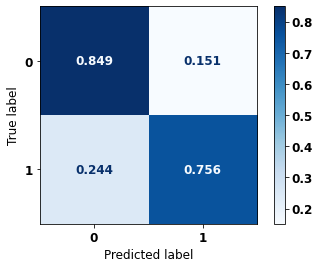
              precision    recall  f1-score   support

           0      0.650     0.849     0.736       510
           1      0.903     0.756     0.823       953

    accuracy                          0.788      1463
   macro avg      0.777     0.802     0.780      1463
weighted avg      0.815     0.788     0.793      1463
[ ]:
display_confusion_matrix(xgb_fora_00_03, X_testOS_12_15, y_testOS_12_15)

              precision    recall  f1-score   support

           0      0.624     0.823     0.710       571
           1      0.902     0.766     0.829      1211

    accuracy                          0.785      1782
   macro avg      0.763     0.795     0.769      1782
weighted avg      0.813     0.785     0.791      1782
[ ]:
display_confusion_matrix(xgb_fora_00_03, X_testOS_16_20, y_testOS_16_20)

              precision    recall  f1-score   support

           0      0.828     0.839     0.833       539
           1      0.800     0.787     0.794       442

    accuracy                          0.815       981
   macro avg      0.814     0.813     0.813       981
weighted avg      0.815     0.815     0.815       981
Random Forest Other states for years 2004 to 2007
[ ]:
display_confusion_matrix(rf_fora_04_07, X_testOS_08_11, y_testOS_08_11)
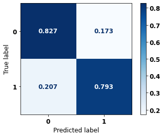
              precision    recall  f1-score   support

           0      0.682     0.827     0.748       510
           1      0.896     0.793     0.841       953

    accuracy                          0.805      1463
   macro avg      0.789     0.810     0.794      1463
weighted avg      0.821     0.805     0.809      1463
[ ]:
display_confusion_matrix(rf_fora_04_07, X_testOS_12_15, y_testOS_12_15)

              precision    recall  f1-score   support

           0      0.642     0.820     0.720       571
           1      0.902     0.784     0.839      1211

    accuracy                          0.796      1782
   macro avg      0.772     0.802     0.780      1782
weighted avg      0.819     0.796     0.801      1782
[ ]:
display_confusion_matrix(rf_fora_04_07, X_testOS_16_20, y_testOS_16_20)

              precision    recall  f1-score   support

           0      0.820     0.837     0.828       539
           1      0.796     0.776     0.786       442

    accuracy                          0.809       981
   macro avg      0.808     0.806     0.807       981
weighted avg      0.809     0.809     0.809       981
XGBoost Other states for years 2004 to 2007
[ ]:
display_confusion_matrix(xgb_fora_04_07, X_testOS_08_11, y_testOS_08_11)
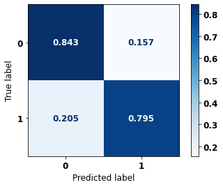
              precision    recall  f1-score   support

           0      0.688     0.843     0.758       510
           1      0.905     0.795     0.846       953

    accuracy                          0.812      1463
   macro avg      0.796     0.819     0.802      1463
weighted avg      0.829     0.812     0.816      1463
[ ]:
display_confusion_matrix(xgb_fora_04_07, X_testOS_12_15, y_testOS_12_15)

              precision    recall  f1-score   support

           0      0.637     0.828     0.720       571
           1      0.906     0.777     0.836      1211

    accuracy                          0.793      1782
   macro avg      0.771     0.803     0.778      1782
weighted avg      0.819     0.793     0.799      1782
[ ]:
display_confusion_matrix(xgb_fora_04_07, X_testOS_16_20, y_testOS_16_20)

              precision    recall  f1-score   support

           0      0.820     0.853     0.836       539
           1      0.812     0.771     0.791       442

    accuracy                          0.817       981
   macro avg      0.816     0.812     0.814       981
weighted avg      0.816     0.817     0.816       981
Random Forest Other states for years 2008 to 2011
[ ]:
display_confusion_matrix(rf_fora_08_11, X_testOS_12_15, y_testOS_12_15)

              precision    recall  f1-score   support

           0      0.665     0.792     0.723       571
           1      0.892     0.812     0.850      1211

    accuracy                          0.805      1782
   macro avg      0.778     0.802     0.786      1782
weighted avg      0.819     0.805     0.809      1782
[ ]:
display_confusion_matrix(rf_fora_08_11, X_testOS_16_20, y_testOS_16_20)

              precision    recall  f1-score   support

           0      0.844     0.805     0.824       539
           1      0.775     0.819     0.796       442

    accuracy                          0.811       981
   macro avg      0.810     0.812     0.810       981
weighted avg      0.813     0.811     0.812       981
XGBoost Other states for years 2008 to 2011
[ ]:
display_confusion_matrix(xgb_fora_08_11, X_testOS_12_15, y_testOS_12_15)
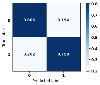
              precision    recall  f1-score   support

           0      0.652     0.806     0.721       571
           1      0.897     0.798     0.844      1211

    accuracy                          0.800      1782
   macro avg      0.775     0.802     0.783      1782
weighted avg      0.819     0.800     0.805      1782
[ ]:
display_confusion_matrix(xgb_fora_08_11, X_testOS_16_20, y_testOS_16_20)

              precision    recall  f1-score   support

           0      0.824     0.814     0.819       539
           1      0.777     0.787     0.782       442

    accuracy                          0.802       981
   macro avg      0.800     0.801     0.801       981
weighted avg      0.803     0.802     0.802       981
Random Forest Other states for years 2012 to 2015
[ ]:
display_confusion_matrix(rf_fora_12_15, X_testOS_16_20, y_testOS_16_20)

              precision    recall  f1-score   support

           0      0.837     0.850     0.843       539
           1      0.813     0.799     0.806       442

    accuracy                          0.827       981
   macro avg      0.825     0.824     0.825       981
weighted avg      0.827     0.827     0.827       981
XGBoost Other states for years 2012 to 2015
[ ]:
display_confusion_matrix(xgb_fora_12_15, X_testOS_16_20, y_testOS_16_20)

              precision    recall  f1-score   support

           0      0.840     0.848     0.844       539
           1      0.812     0.803     0.808       442

    accuracy                          0.828       981
   macro avg      0.826     0.826     0.826       981
weighted avg      0.828     0.828     0.828       981
Fifth approach
Approach with grouped years and without the columns EC and HORMONIO.
Preprocessing
Now we are going to divide the data into training and testing, and then do the preprocessing in both datasets to perform the training of the models and their evaluation. We will use the years grouped too, resulting in 5 datasets for SP and more 5 for other states.
First, it is necessary to define the columns that will be used as features and the label. We will not use some columns of the datasets: UFRESID, because we already have the division between SP and other states in the two datasets.
It was chosen to keep the column IDADE, so we will not use the FAIXAETAR, as well as the column ECGRUP and not the column EC. Finally, the other columns contained in the list list_drop are possible labels, so they will not be used as features for machine learning models.
[ ]:
list_drop = ['UFRESID', 'FAIXAETAR', 'ULTICONS', 'ULTIDIAG', 'ULTITRAT',
             'obito_geral', 'obito_cancer', 'vivo_ano1', 'vivo_ano5',
             'ULTINFO', 'EC', 'HORMONIO']

# 'RECNENHUM', 'RECLOCAL', 'RECREGIO', 'REC01', 'REC02', 'REC03', 'RECDIST'

lb = 'vivo_ano3'
A function was created to perform the preprocessing, preprocessing, that uses the other functions created, get_train_test (divides the dataset into train and test sets), train_preprocessing (do the preprocessing of the train set) and test_preprocessing (do the preprocessing of the test set).
The process will be done 5 times for SP and other states, using the datasets with grouped years.
To see the complete function go to the functions section.
SP
[ ]:
X_trainSP_00_03, X_testSP_00_03, y_trainSP_00_03, y_testSP_00_03, feat_SP_00_03 = preprocessing(df_SP_ano3, list_drop, lb,
                                                                                                group_years=True,
                                                                                                first_year=2000,
                                                                                                last_year=2003,
                                                                                                random_state=seed,
                                                                                                balance_data=False,
                                                                                                encoder_type='LabelEncoder',
                                                                                                norm_name='StandardScaler')
X_train = (45987, 64), X_test = (15329, 64)
y_train = (45987,), y_test = (15329,)
[ ]:
X_trainSP_04_07, X_testSP_04_07, y_trainSP_04_07, y_testSP_04_07, feat_SP_04_07 = preprocessing(df_SP_ano3, list_drop, lb,
                                                                                                group_years=True,
                                                                                                first_year=2004,
                                                                                                last_year=2007,
                                                                                                random_state=seed,
                                                                                                balance_data=False,
                                                                                                encoder_type='LabelEncoder',
                                                                                                norm_name='StandardScaler')
X_train = (57801, 64), X_test = (19267, 64)
y_train = (57801,), y_test = (19267,)
[ ]:
X_trainSP_08_11, X_testSP_08_11, y_trainSP_08_11, y_testSP_08_11, feat_SP_08_11 = preprocessing(df_SP_ano3, list_drop, lb,
                                                                                                group_years=True,
                                                                                                first_year=2008,
                                                                                                last_year=2011,
                                                                                                random_state=seed,
                                                                                                balance_data=False,
                                                                                                encoder_type='LabelEncoder',
                                                                                                norm_name='StandardScaler')
X_train = (77655, 64), X_test = (25886, 64)
y_train = (77655,), y_test = (25886,)
[ ]:
X_trainSP_12_15, X_testSP_12_15, y_trainSP_12_15, y_testSP_12_15, feat_SP_12_15 = preprocessing(df_SP_ano3, list_drop, lb,
                                                                                                group_years=True,
                                                                                                first_year=2012,
                                                                                                last_year=2015,
                                                                                                random_state=seed,
                                                                                                balance_data=False,
                                                                                                encoder_type='LabelEncoder',
                                                                                                norm_name='StandardScaler')
X_train = (89562, 64), X_test = (29854, 64)
y_train = (89562,), y_test = (29854,)
[ ]:
X_trainSP_16_21, X_testSP_16_21, y_trainSP_16_21, y_testSP_16_21, feat_SP_16_21 = preprocessing(df_SP_ano3, list_drop, lb,
                                                                                                group_years=True,
                                                                                                first_year=2016,
                                                                                                last_year=2021,
                                                                                                random_state=seed,
                                                                                                balance_data=False,
                                                                                                encoder_type='LabelEncoder',
                                                                                                norm_name='StandardScaler')
X_train = (35880, 64), X_test = (11961, 64)
y_train = (35880,), y_test = (11961,)
Other states
[ ]:
X_trainOS_00_03, X_testOS_00_03, y_trainOS_00_03, y_testOS_00_03, feat_OS_00_03 = preprocessing(df_fora_ano3, list_drop, lb,
group_years=True,
first_year=2000,
last_year=2003,
random_state=seed,
balance_data=False,
encoder_type='LabelEncoder',
norm_name='StandardScaler')
X_train = (2631, 64), X_test = (877, 64)
y_train = (2631,), y_test = (877,)
[ ]:
X_trainOS_04_07, X_testOS_04_07, y_trainOS_04_07, y_testOS_04_07, feat_OS_04_07 = preprocessing(df_fora_ano3, list_drop, lb,
group_years=True,
first_year=2004,
last_year=2007,
random_state=seed,
balance_data=False,
encoder_type='LabelEncoder',
norm_name='StandardScaler')
X_train = (3652, 64), X_test = (1218, 64)
y_train = (3652,), y_test = (1218,)
[ ]:
X_trainOS_08_11, X_testOS_08_11, y_trainOS_08_11, y_testOS_08_11, feat_OS_08_11 = preprocessing(df_fora_ano3, list_drop, lb,
group_years=True,
first_year=2008,
last_year=2011,
random_state=seed,
balance_data=False,
encoder_type='LabelEncoder',
norm_name='StandardScaler')
X_train = (4387, 64), X_test = (1463, 64)
y_train = (4387,), y_test = (1463,)
[ ]:
X_trainOS_12_15, X_testOS_12_15, y_trainOS_12_15, y_testOS_12_15, feat_OS_12_15 = preprocessing(df_fora_ano3, list_drop, lb,
group_years=True,
first_year=2012,
last_year=2015,
random_state=seed,
balance_data=False,
encoder_type='LabelEncoder',
norm_name='StandardScaler')
X_train = (5346, 64), X_test = (1782, 64)
y_train = (5346,), y_test = (1782,)
[ ]:
X_trainOS_16_20, X_testOS_16_20, y_trainOS_16_20, y_testOS_16_20, feat_OS_16_20 = preprocessing(df_fora_ano3, list_drop, lb,
group_years=True,
first_year=2016,
last_year=2020,
random_state=seed,
balance_data=False,
encoder_type='LabelEncoder',
norm_name='StandardScaler')
X_train = (2943, 64), X_test = (981, 64)
y_train = (2943,), y_test = (981,)
Training and evaluation of the models
After dividing the data into training and testing, using the encoder and normalizing, the data is ready to be used by the machine learning models.
Random Forest
The first model is the Random Forest, the random_state will be used as a parameter, to obtain the same training values of the model every time it is runned.
The hyperparameter class_weight was used because the models have difficulty to learn the class with fewer examples.
SP
[ ]:
# SP - 2000 to 2003
rf_sp_00_03 = RandomForestClassifier(random_state=seed,
class_weight={0:1.405, 1:1},
criterion='entropy',
max_depth=10)
rf_sp_00_03.fit(X_trainSP_00_03, y_trainSP_00_03)
RandomForestClassifier(class_weight={0: 1.405, 1: 1}, criterion='entropy',
max_depth=10, random_state=10)
[ ]:
display_confusion_matrix(rf_sp_00_03, X_testSP_00_03, y_testSP_00_03)

precision recall f1-score support
0 0.738 0.795 0.765 6483
1 0.841 0.793 0.816 8846
accuracy 0.794 15329
macro avg 0.789 0.794 0.791 15329
weighted avg 0.797 0.794 0.795 15329
The confusion matrix obtained for the Random Forest, with SP data from 2000 to 2003, shows a good performance of the model, with 79% of accuracy.
[ ]:
show_tree(rf_sp_00_03, feat_SP_00_03, 2)
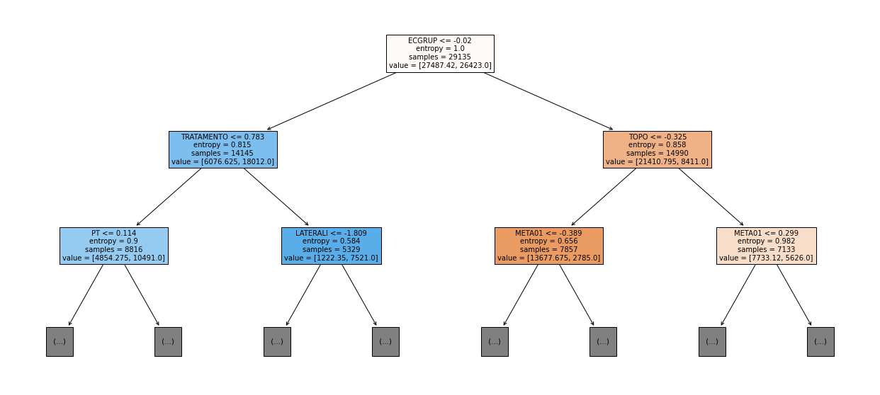
[ ]:
plot_roc_curve(rf_sp_00_03, X_trainSP_00_03, X_testSP_00_03, y_trainSP_00_03, y_testSP_00_03)

[ ]:
plot_feat_importances(rf_sp_00_03, feat_SP_00_03)
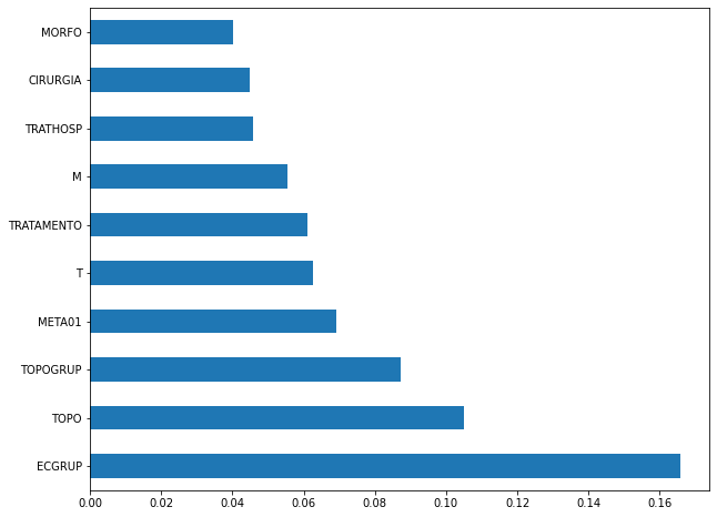
The four most important features in the model were
ECGRUP,TOPO,TOPOGRUP, andMETA01.
[ ]:
plot_shap_values(rf_sp_00_03, X_testSP_00_03, feat_SP_00_03)
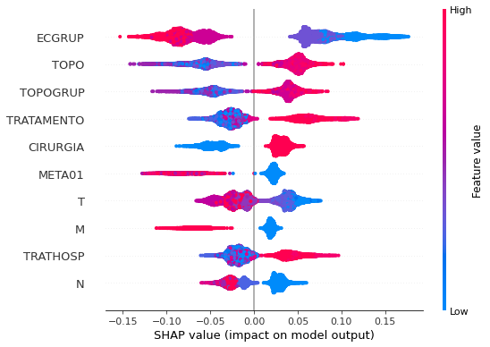
Note that larger values of the ECGRUP column, shown in pink, have more influence for the model’s prediction to be class 0, smaller values have greater weight for the prediction to be class 1. This behavior was expected, because the higher the clinical stage, worse is the stage of cancer.
The other columns shown follow the same logic.
[ ]:
# SP - 2004 to 2007
rf_sp_04_07 = RandomForestClassifier(random_state=seed,
class_weight={0:1.62, 1:1},
criterion='entropy',
max_depth=10)
rf_sp_04_07.fit(X_trainSP_04_07, y_trainSP_04_07)
RandomForestClassifier(class_weight={0: 1.62, 1: 1}, criterion='entropy',
max_depth=10, random_state=10)
[ ]:
display_confusion_matrix(rf_sp_04_07, X_testSP_04_07, y_testSP_04_07)

precision recall f1-score support
0 0.724 0.801 0.760 7568
1 0.862 0.802 0.831 11699
accuracy 0.802 19267
macro avg 0.793 0.802 0.796 19267
weighted avg 0.808 0.802 0.803 19267
The confusion matrix obtained for the Random Forest, with SP data from 2004 to 2007, shows a good performance of the model, with 80% of accuracy.
[ ]:
show_tree(rf_sp_04_07, feat_SP_04_07, 2)
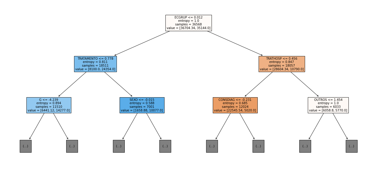
[ ]:
plot_roc_curve(rf_sp_04_07, X_trainSP_04_07, X_testSP_04_07, y_trainSP_04_07, y_testSP_04_07)
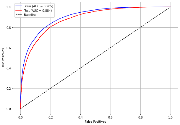
[ ]:
plot_feat_importances(rf_sp_04_07, feat_SP_04_07)
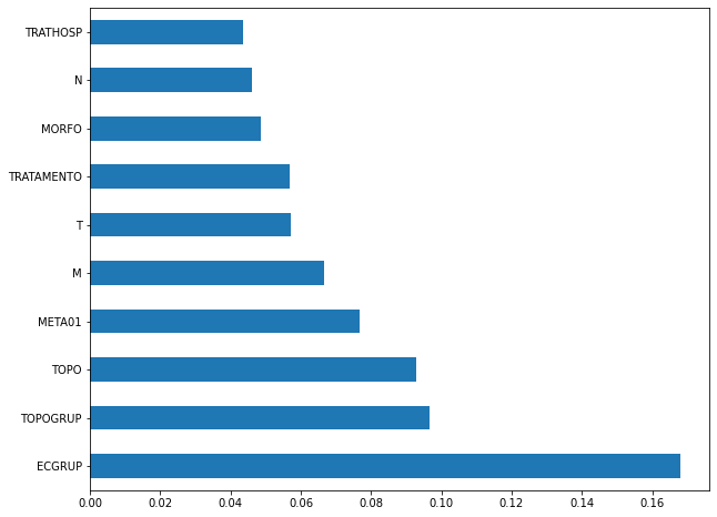
The four most important features in the model were
ECGRUP,TOPOGRUP,TOPOandMETA01.
[ ]:
plot_shap_values(rf_sp_04_07, X_testSP_04_07, feat_SP_04_07)
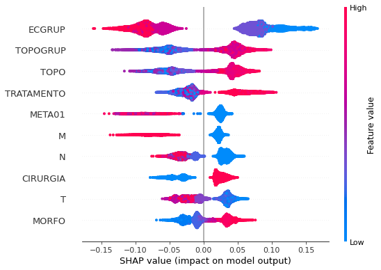
Note that larger values of the ECGRUP column, shown in pink, have more influence for the model’s prediction to be class 0, smaller values have greater weight for the prediction to be class 1. This behavior was expected, because the higher the clinical stage, worse is the stage of cancer.
The other columns shown follow the same logic.
[ ]:
# SP - 2008 to 2011
rf_sp_08_11 = RandomForestClassifier(random_state=seed,
class_weight={0:1.85, 1:1},
criterion='entropy',
max_depth=10)
rf_sp_08_11.fit(X_trainSP_08_11, y_trainSP_08_11)
RandomForestClassifier(class_weight={0: 1.85, 1: 1}, criterion='entropy',
max_depth=10, random_state=10)
[ ]:
display_confusion_matrix(rf_sp_08_11, X_testSP_08_11, y_testSP_08_11)

precision recall f1-score support
0 0.717 0.811 0.761 9635
1 0.879 0.810 0.843 16251
accuracy 0.811 25886
macro avg 0.798 0.811 0.802 25886
weighted avg 0.818 0.811 0.813 25886
The confusion matrix obtained for the Random Forest, with SP data from 2008 to 2011, shows a good performance of the model, with 81% of accuracy.
[ ]:
show_tree(rf_sp_08_11, feat_SP_08_11, 2)
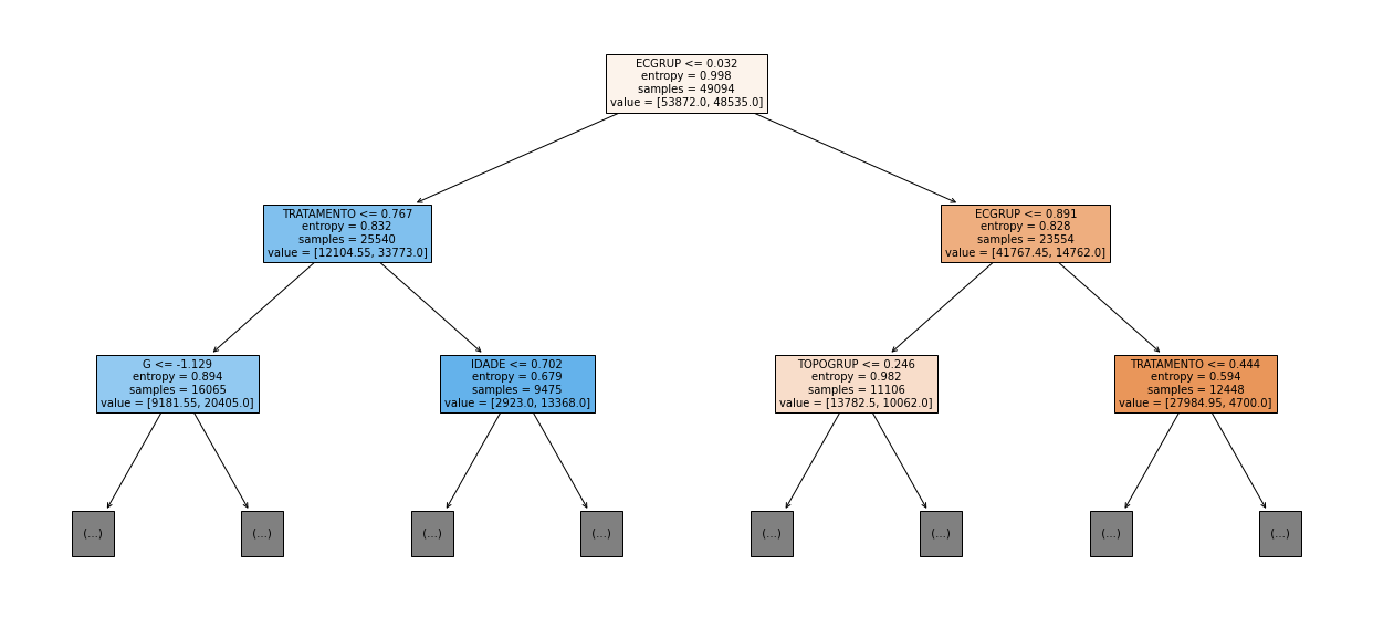
[ ]:
plot_roc_curve(rf_sp_08_11, X_trainSP_08_11, X_testSP_08_11, y_trainSP_08_11, y_testSP_08_11)
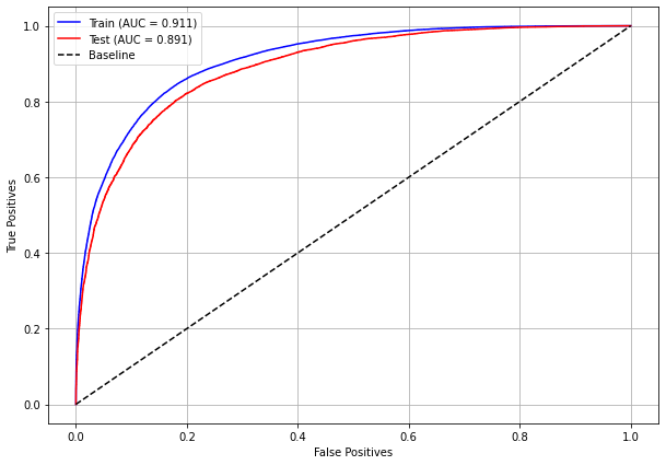
[ ]:
plot_feat_importances(rf_sp_08_11, feat_SP_08_11)
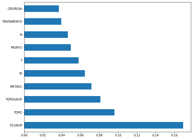
The four most important features in the model were
ECGRUP,TOPO,TOPOGRUPandMETA01.
[ ]:
plot_shap_values(rf_sp_08_11, X_testSP_08_11, feat_SP_08_11)
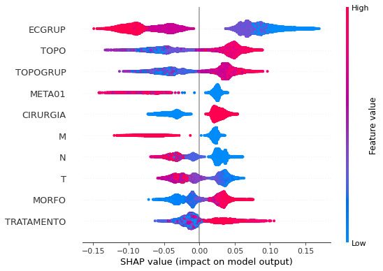
Note that larger values of the ECGRUP column, shown in pink, have more influence for the model’s prediction to be class 0, smaller values have greater weight for the prediction to be class 1. This behavior was expected, because the higher the clinical stage, worse is the stage of cancer.
The other columns shown follow the same logic.
[ ]:
# SP - 2012 to 2015
rf_sp_12_15 = RandomForestClassifier(random_state=seed,
class_weight={0:2.03, 1:1},
criterion='entropy',
max_depth=10)
rf_sp_12_15.fit(X_trainSP_12_15, y_trainSP_12_15)
RandomForestClassifier(class_weight={0: 2.03, 1: 1}, criterion='entropy',
max_depth=10, random_state=10)
[ ]:
display_confusion_matrix(rf_sp_12_15, X_testSP_12_15, y_testSP_12_15)

precision recall f1-score support
0 0.703 0.811 0.753 10563
1 0.887 0.812 0.848 19291
accuracy 0.812 29854
macro avg 0.795 0.812 0.800 29854
weighted avg 0.822 0.812 0.814 29854
The confusion matrix obtained for the Random Forest, with SP data from 2012 to 2015, shows a good performance of the model with 81% of accuracy.
[ ]:
show_tree(rf_sp_12_15, feat_SP_12_15, 2)
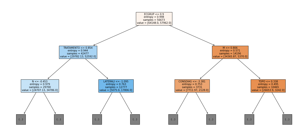
[ ]:
plot_roc_curve(rf_sp_12_15, X_trainSP_12_15, X_testSP_12_15, y_trainSP_12_15, y_testSP_12_15)
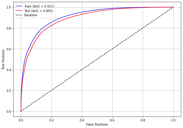
[ ]:
plot_feat_importances(rf_sp_12_15, feat_SP_12_15)
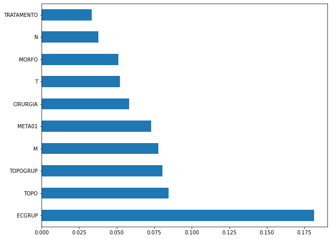
The four most important features in the model were
ECGRUP,TOPO,TOPOGRUPandM.
[ ]:
plot_shap_values(rf_sp_12_15, X_testSP_12_15, feat_SP_12_15)
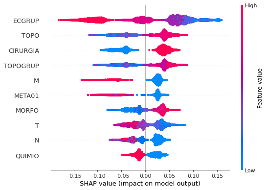
Note that larger values of the ECGRUP column, shown in pink, have more influence for the model’s prediction to be class 0, smaller values have greater weight for the prediction to be class 1. This behavior was expected, because the higher the clinical stage, worse is the stage of cancer.
The other columns shown follow the same logic.
[ ]:
# SP - 2016 to 2021
rf_sp_16_21 = RandomForestClassifier(random_state=seed,
class_weight={0:1, 1:1.25},
criterion='entropy',
max_depth=10)
rf_sp_16_21.fit(X_trainSP_16_21, y_trainSP_16_21)
RandomForestClassifier(class_weight={0: 1, 1: 1.25}, criterion='entropy',
max_depth=10, random_state=10)
[ ]:
display_confusion_matrix(rf_sp_16_21, X_testSP_16_21, y_testSP_16_21)

precision recall f1-score support
0 0.870 0.838 0.854 6773
1 0.798 0.837 0.817 5188
accuracy 0.837 11961
macro avg 0.834 0.837 0.835 11961
weighted avg 0.839 0.837 0.838 11961
The confusion matrix obtained for the Random Forest, with SP data from 2016 to 2021, shows a good performance of the model, with 84% of accuracy.
[ ]:
show_tree(rf_sp_16_21, feat_SP_16_21, 2)
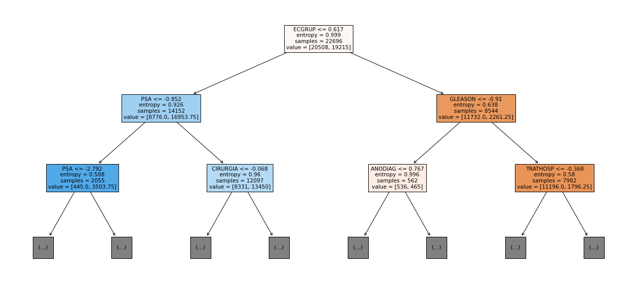
[ ]:
plot_roc_curve(rf_sp_16_21, X_trainSP_16_21, X_testSP_16_21, y_trainSP_16_21, y_testSP_16_21)
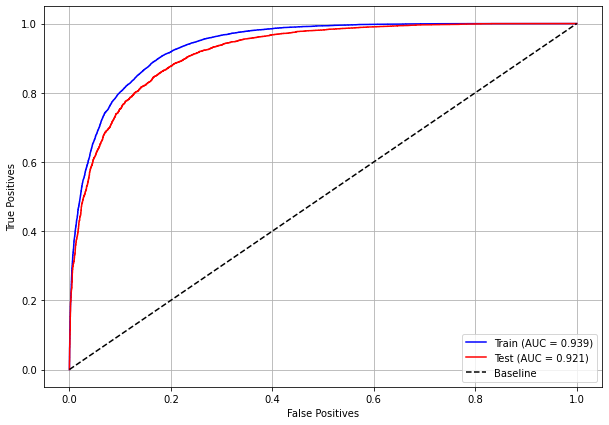
[ ]:
plot_feat_importances(rf_sp_16_21, feat_SP_16_21)
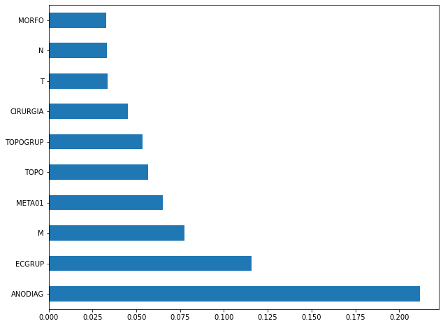
The four most important features in the model were
ANODIAG,ECGRUP,M, andMETA01.
[ ]:
plot_shap_values(rf_sp_16_21, X_testSP_16_21, feat_SP_16_21)
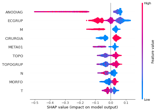
Note that larger values of the ANODIAG column, shown in pink, have more influence for the model’s prediction to be class 0, smaller values have greater weight for the prediction to be class 1.
The other columns shown follow the same logic.
Other states
[ ]:
# Other states - 2000 to 2003
rf_fora_00_03 = RandomForestClassifier(random_state=seed,
class_weight={0:1.86, 1:1},
criterion='entropy',
max_depth=6)
rf_fora_00_03.fit(X_trainOS_00_03, y_trainOS_00_03)
RandomForestClassifier(class_weight={0: 1.86, 1: 1}, criterion='entropy',
max_depth=6, random_state=10)
[ ]:
display_confusion_matrix(rf_fora_00_03, X_testOS_00_03, y_testOS_00_03)

precision recall f1-score support
0 0.684 0.764 0.721 351
1 0.829 0.764 0.795 526
accuracy 0.764 877
macro avg 0.756 0.764 0.758 877
weighted avg 0.771 0.764 0.766 877
The confusion matrix obtained for the Random Forest, with other states data from 2000 to 2003, also shows a good performance of the model, and we have a balanced main diagonal with 76% of accuracy.
[ ]:
show_tree(rf_fora_00_03, feat_OS_00_03, 2)
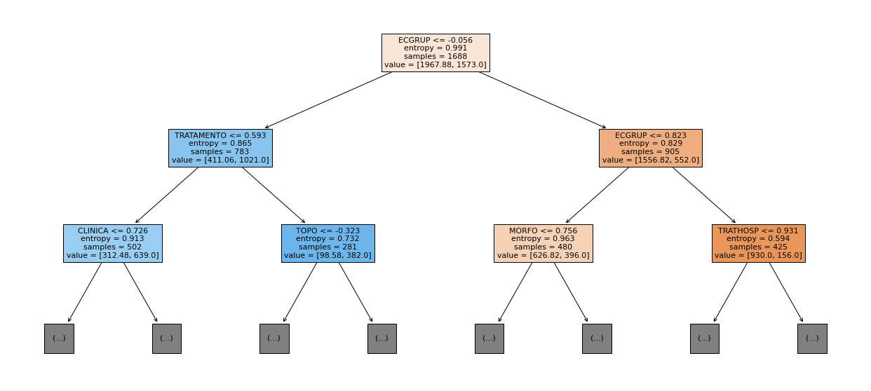
[ ]:
plot_roc_curve(rf_fora_00_03, X_trainOS_00_03, X_testOS_00_03, y_trainOS_00_03, y_testOS_00_03)
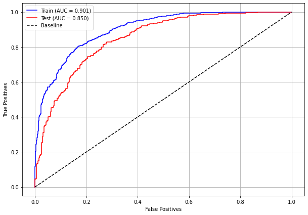
[ ]:
plot_feat_importances(rf_fora_00_03, feat_OS_00_03)
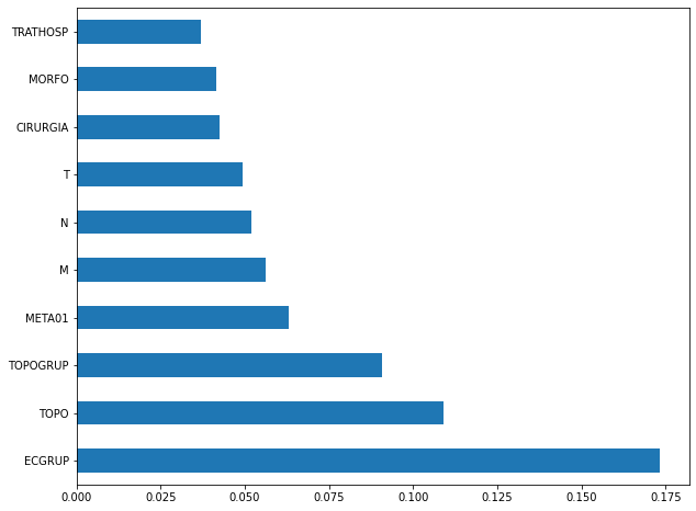
The four most important features in the model were
ECGRUP,TOPO,TOPOGRUPandMETA01.
[ ]:
plot_shap_values(rf_fora_00_03, X_testOS_00_03, feat_OS_00_03)
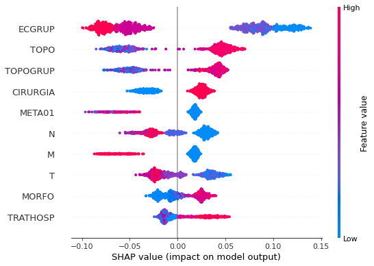
Note that larger values of the ECGRUP column, shown in pink, have more influence for the model’s prediction to be class 0, smaller values have greater weight for the prediction to be class 1. This behavior was expected, because the higher the clinical stage, worse is the stage of cancer.
The other columns shown follow the same logic.
[ ]:
# Other states - 2004 to 2007
rf_fora_04_07 = RandomForestClassifier(random_state=seed,
class_weight={0:1.75, 1:1},
criterion='entropy',
max_depth=6)
rf_fora_04_07.fit(X_trainOS_04_07, y_trainOS_04_07)
RandomForestClassifier(class_weight={0: 1.75, 1: 1}, criterion='entropy',
max_depth=6, random_state=10)
[ ]:
display_confusion_matrix(rf_fora_04_07, X_testOS_04_07, y_testOS_04_07)

precision recall f1-score support
0 0.708 0.808 0.754 443
1 0.881 0.809 0.843 775
accuracy 0.809 1218
macro avg 0.794 0.809 0.799 1218
weighted avg 0.818 0.809 0.811 1218
The confusion matrix obtained for the Random Forest, with other states data from 2004 to 2007, also shows a good performance of the model, with 81% of accuracy.
[ ]:
show_tree(rf_fora_04_07, feat_OS_04_07, 2)
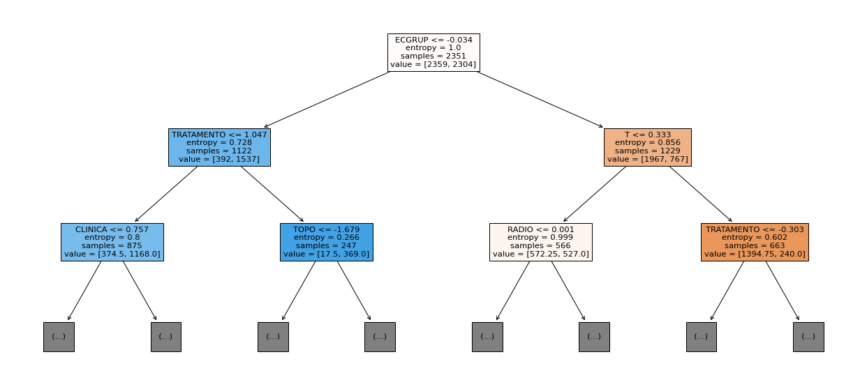
[ ]:
plot_roc_curve(rf_fora_04_07, X_trainOS_04_07, X_testOS_04_07, y_trainOS_04_07, y_testOS_04_07)
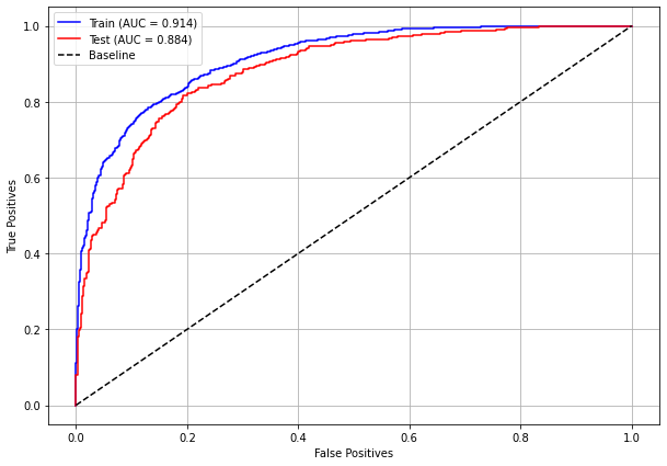
[ ]:
plot_feat_importances(rf_fora_04_07, feat_OS_04_07)
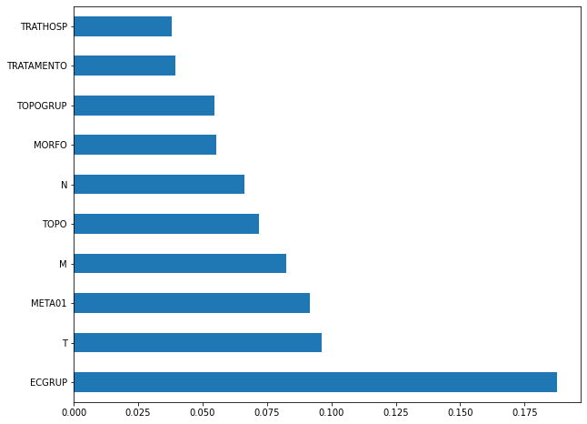
The four most important features in the model were
ECGRUP,T,META01andM.
[ ]:
plot_shap_values(rf_fora_04_07, X_testOS_04_07, feat_OS_04_07)
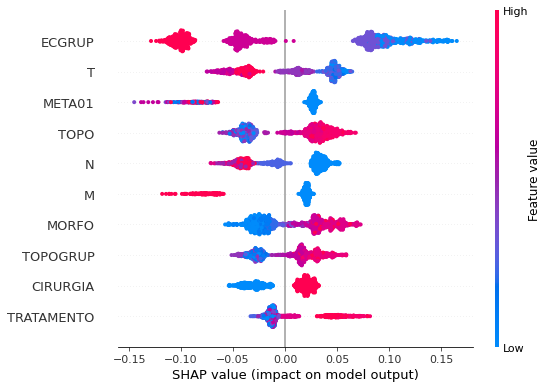
Note that larger values of the ECGRUP column, shown in pink, have more influence for the model’s prediction to be class 0, smaller values have greater weight for the prediction to be class 1. This behavior was expected, because the higher the clinical stage, worse is the stage of cancer.
The other columns shown follow the same logic.
[ ]:
# Other states - 2008 to 2011
rf_fora_08_11 = RandomForestClassifier(random_state=seed,
class_weight={0:2.32, 1:1},
criterion='entropy',
max_depth=6)
rf_fora_08_11.fit(X_trainOS_08_11, y_trainOS_08_11)
RandomForestClassifier(class_weight={0: 2.32, 1: 1}, criterion='entropy',
max_depth=6, random_state=10)
[ ]:
display_confusion_matrix(rf_fora_08_11, X_testOS_08_11, y_testOS_08_11)

precision recall f1-score support
0 0.711 0.822 0.763 510
1 0.896 0.822 0.857 953
accuracy 0.822 1463
macro avg 0.804 0.822 0.810 1463
weighted avg 0.832 0.822 0.824 1463
The confusion matrix obtained for the Random Forest, with other states data from 2008 to 2011, also shows a good performance of the model, presenting 82% of accuracy.
[ ]:
show_tree(rf_fora_08_11, feat_OS_08_11, 2)
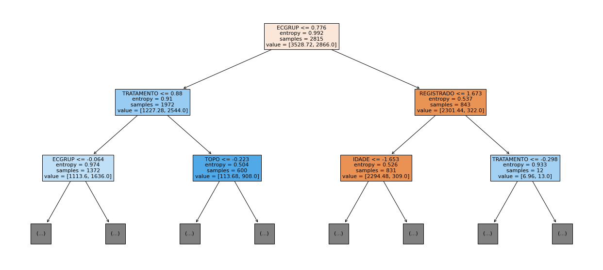
[ ]:
plot_roc_curve(rf_fora_08_11, X_trainOS_08_11, X_testOS_08_11, y_trainOS_08_11, y_testOS_08_11)
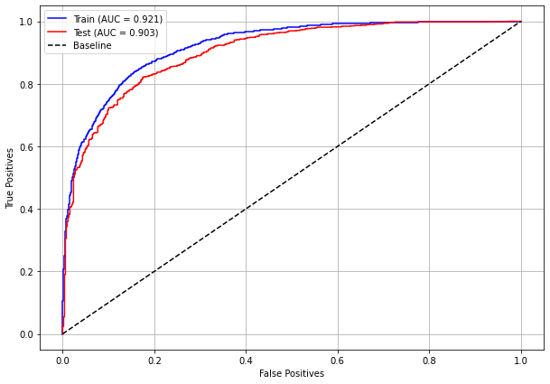
[ ]:
plot_feat_importances(rf_fora_08_11, feat_OS_08_11)
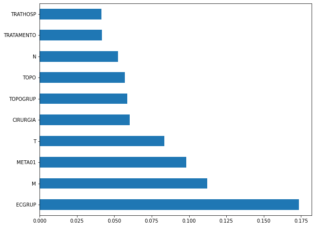
The four most important features in the model were
ECGRUP,M,META01andT.
[ ]:
plot_shap_values(rf_fora_08_11, X_testOS_08_11, feat_OS_08_11)
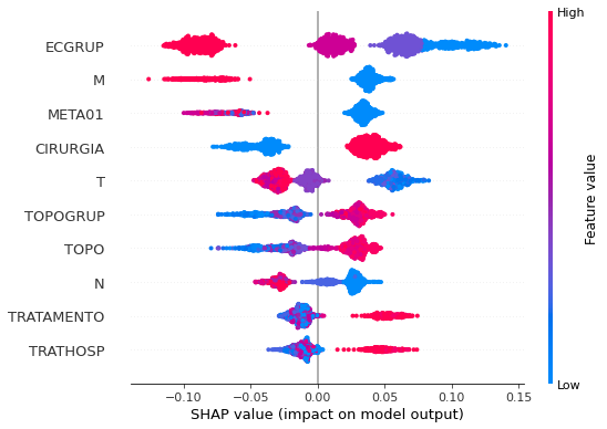
Note that larger values of the ECGRUP column, shown in pink, have more influence for the model’s prediction to be class 0, smaller values have greater weight for the prediction to be class 1. This behavior was expected, because the higher the clinical stage, worse is the stage of cancer.
The other columns shown follow the same logic.
[ ]:
# Other states - 2012 to 2015
rf_fora_12_15 = RandomForestClassifier(random_state=seed,
class_weight={0:3.21, 1:1},
criterion='entropy',
max_depth=8)
rf_fora_12_15.fit(X_trainOS_12_15, y_trainOS_12_15)
RandomForestClassifier(class_weight={0: 3.21, 1: 1}, criterion='entropy',
max_depth=8, random_state=10)
[ ]:
display_confusion_matrix(rf_fora_12_15, X_testOS_12_15, y_testOS_12_15)

precision recall f1-score support
0 0.673 0.814 0.737 571
1 0.903 0.813 0.856 1211
accuracy 0.814 1782
macro avg 0.788 0.814 0.796 1782
weighted avg 0.829 0.814 0.818 1782
The confusion matrix obtained for the Random Forest, with other states data from 2012 to 2015, also shows a good performance of the model, presenting 81% of accuracy.
[ ]:
show_tree(rf_fora_12_15, feat_OS_12_15, 2)
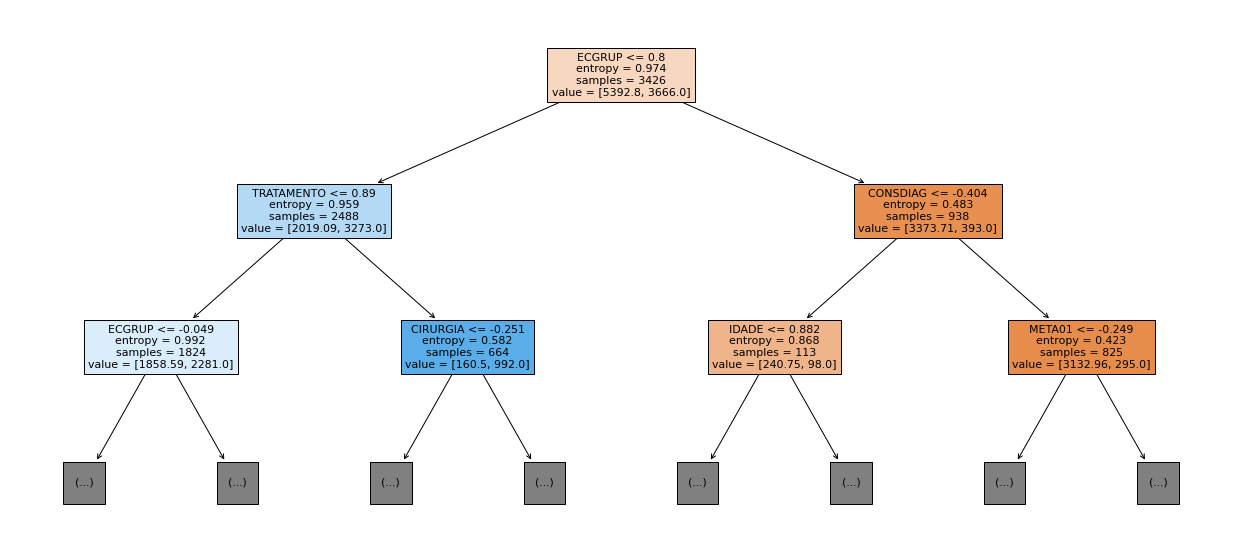
[ ]:
plot_roc_curve(rf_fora_12_15, X_trainOS_12_15, X_testOS_12_15, y_trainOS_12_15, y_testOS_12_15)
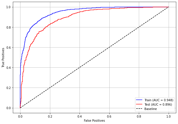
[ ]:
plot_feat_importances(rf_fora_12_15, feat_OS_12_15)
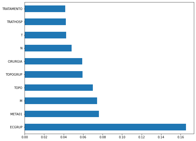
The four most important features in the model were
ECGRUP,META01,MandTOPO.
[ ]:
plot_shap_values(rf_fora_12_15, X_testOS_12_15, feat_OS_12_15)
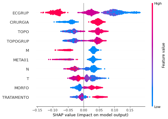
Note that larger values of the ECGRUP column, shown in pink, have more influence for the model’s prediction to be class 0, smaller values have greater weight for the prediction to be class 1. This behavior was expected, because the higher the clinical stage, worse is the stage of cancer.
The other columns shown follow the same logic.
[ ]:
# Other states - 2016 to 2020
rf_fora_16_20 = RandomForestClassifier(random_state=seed,
class_weight={0:1, 1:1.09},
criterion='entropy',
max_depth=8)
rf_fora_16_20.fit(X_trainOS_16_20, y_trainOS_16_20)
RandomForestClassifier(class_weight={0: 1, 1: 1.09}, criterion='entropy',
max_depth=8, random_state=10)
[ ]:
display_confusion_matrix(rf_fora_16_20, X_testOS_16_20, y_testOS_16_20)

precision recall f1-score support
0 0.872 0.848 0.860 539
1 0.821 0.848 0.834 442
accuracy 0.848 981
macro avg 0.846 0.848 0.847 981
weighted avg 0.849 0.848 0.848 981
The confusion matrix obtained for the Random Forest, with other states data from 2016 to 2020, also shows a good performance of the model, presenting 85% of accuracy.
[ ]:
show_tree(rf_fora_16_20, feat_OS_16_20, 3)
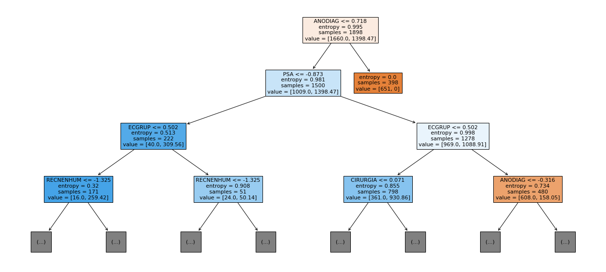
[ ]:
plot_roc_curve(rf_fora_16_20, X_trainOS_16_20, X_testOS_16_20, y_trainOS_16_20, y_testOS_16_20)

[ ]:
plot_feat_importances(rf_fora_16_20, feat_OS_16_20)
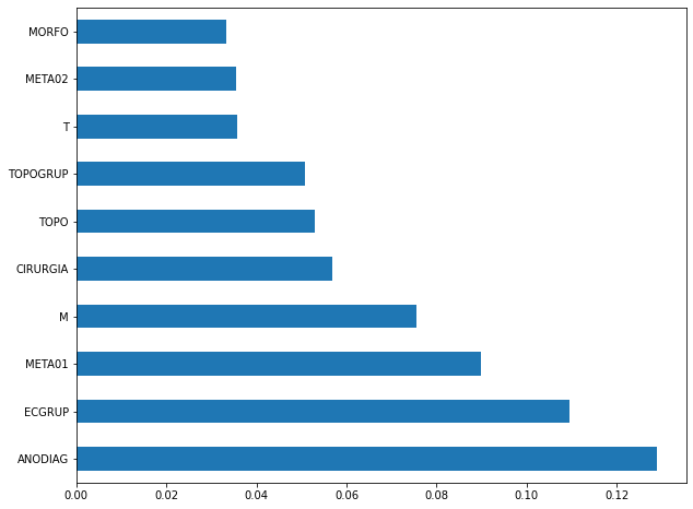
The four most important features in the model were
ANODIAG,ECGRUP,META01andM.
[ ]:
plot_shap_values(rf_fora_16_20, X_testOS_16_20, feat_OS_16_20)
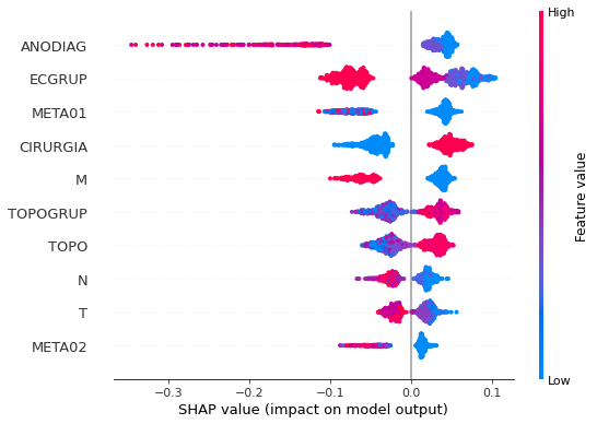
Note that larger values of the ANODIAG column, shown in pink, have more influence for the model’s prediction to be class 0, smaller values have greater weight for the prediction to be class 1.
The other columns shown follow the same logic.
XGBoost
The training of the XGBoost models follows the same pattern with random_state. The hyperparameter scale_pos_weight was also used in some trainings, in order to obtain a balanced main diagonal in the confusion matrix.
The hyperparameter max_depth was chosen as 10 because the default value for this hyperparameter is 3, a low value for the amount of data we have.
SP
[ ]:
# SP - 2000 to 2003
xgb_sp_00_03 = XGBClassifier(max_depth=8,
random_state=seed,
scale_pos_weight=0.7)
xgb_sp_00_03.fit(X_trainSP_00_03, y_trainSP_00_03)
XGBClassifier(max_depth=8, random_state=10, scale_pos_weight=0.7)
[ ]:
display_confusion_matrix(xgb_sp_00_03, X_testSP_00_03, y_testSP_00_03)

precision recall f1-score support
0 0.755 0.809 0.781 6483
1 0.852 0.808 0.830 8846
accuracy 0.808 15329
macro avg 0.804 0.809 0.805 15329
weighted avg 0.811 0.808 0.809 15329
The confusion matrix obtained for the XGBoost, with SP data from 2000 to 2003, shows a good performance of the model, here with 81% of accuracy.
[ ]:
plot_roc_curve(xgb_sp_00_03, X_trainSP_00_03, X_testSP_00_03, y_trainSP_00_03, y_testSP_00_03)
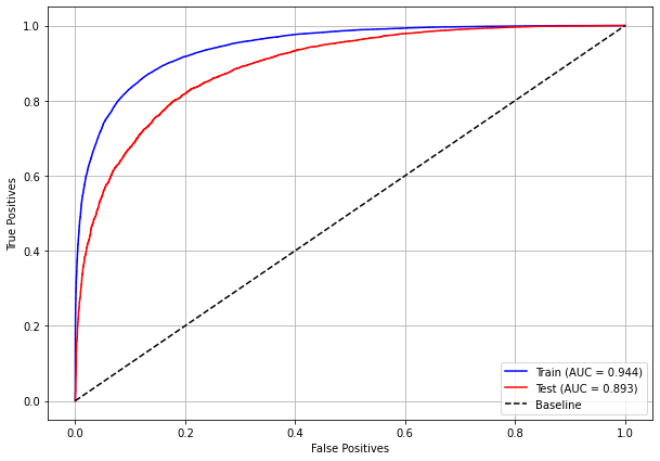
[ ]:
plot_feat_importances(xgb_sp_00_03, feat_SP_00_03)
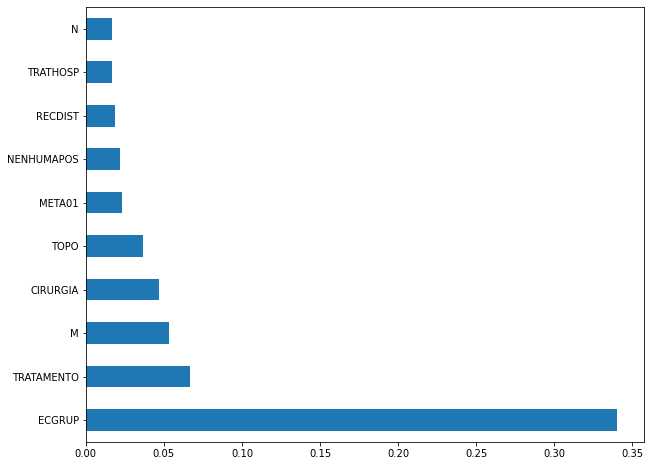
Here we noticed that the most used feature was
ECGRUP, with a lot advantage over the others. Following we haveTRATAMENTO,MandCIRURGIA.
[ ]:
plot_shap_values(xgb_sp_00_03, X_testSP_00_03, feat_SP_00_03)
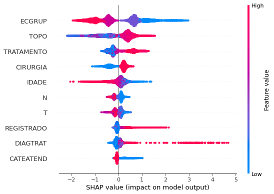
Note that larger values of the ECGRUP column, shown in pink, have more influence for the model’s prediction to be class 0, smaller values have greater weight for the prediction to be class 1. This behavior was expected, because the higher the clinical stage, worse is the stage of cancer.
The other columns shown follow the same logic.
[ ]:
# SP - 2004 to 2007
xgb_sp_04_07 = XGBClassifier(max_depth=8,
random_state=seed,
scale_pos_weight=0.619)
xgb_sp_04_07.fit(X_trainSP_04_07, y_trainSP_04_07)
XGBClassifier(max_depth=8, random_state=10, scale_pos_weight=0.619)
[ ]:
display_confusion_matrix(xgb_sp_04_07, X_testSP_04_07, y_testSP_04_07)

precision recall f1-score support
0 0.744 0.819 0.779 7568
1 0.874 0.818 0.845 11699
accuracy 0.818 19267
macro avg 0.809 0.818 0.812 19267
weighted avg 0.823 0.818 0.819 19267
The confusion matrix obtained for the XGBoost, with SP data from 2004 to 2007, shows a good performance of the model, with 82% of accuracy.
[ ]:
plot_roc_curve(xgb_sp_04_07, X_trainSP_04_07, X_testSP_04_07, y_trainSP_04_07, y_testSP_04_07)

[ ]:
plot_feat_importances(xgb_sp_04_07, feat_SP_04_07)
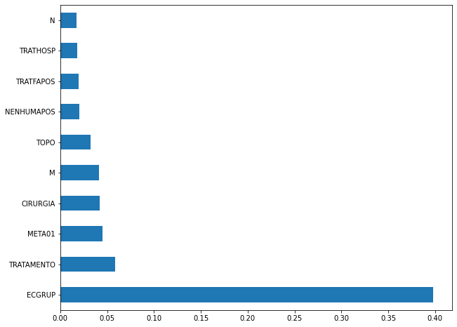
Here we noticed that the most used feature was
ECGRUP, with a good advantage over the others. Following we haveTRATAMENTO,META01andCIRURGIA.
[ ]:
plot_shap_values(xgb_sp_04_07, X_testSP_04_07, feat_SP_04_07)
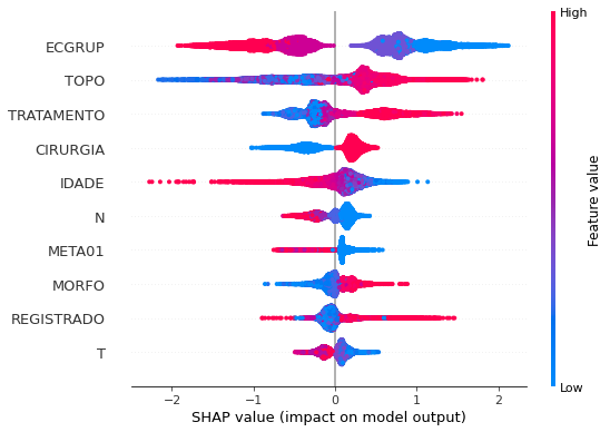
Note that larger values of the ECGRUP column, shown in pink, have more influence for the model’s prediction to be class 0, smaller values have greater weight for the prediction to be class 1. This behavior was expected, because the higher the clinical stage, worse is the stage of cancer.
The other columns shown follow the same logic.
[ ]:
# SP - 2008 to 2011
xgb_sp_08_11 = XGBClassifier(max_depth=8,
scale_pos_weight=0.55,
random_state=seed)
xgb_sp_08_11.fit(X_trainSP_08_11, y_trainSP_08_11)
XGBClassifier(max_depth=8, random_state=10, scale_pos_weight=0.55)
[ ]:
display_confusion_matrix(xgb_sp_08_11, X_testSP_08_11, y_testSP_08_11)

precision recall f1-score support
0 0.738 0.827 0.780 9635
1 0.889 0.826 0.857 16251
accuracy 0.826 25886
macro avg 0.814 0.826 0.818 25886
weighted avg 0.833 0.826 0.828 25886
The confusion matrix obtained for the XGBoost, with SP data from 2008 to 2011, shows a good performance of the model, with 83% of accuracy.
[ ]:
plot_roc_curve(xgb_sp_08_11, X_trainSP_08_11, X_testSP_08_11, y_trainSP_08_11, y_testSP_08_11)

[ ]:
plot_feat_importances(xgb_sp_08_11, feat_SP_08_11)
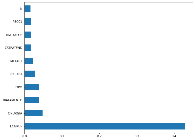
Here we noticed that the most used feature was
ECGRUP, with a good advantage over the others. Following we haveCIRURGIA,TRATAMENTOandTOPO.
[ ]:
plot_shap_values(xgb_sp_08_11, X_testSP_08_11, feat_SP_08_11)
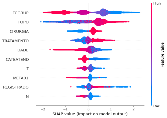
Note that larger values of the ECGRUP column, shown in pink, have more influence for the model’s prediction to be class 0, smaller values have greater weight for the prediction to be class 1. This behavior was expected, because the higher the clinical stage, worse is the stage of cancer.
The other columns shown follow the same logic.
[ ]:
# SP - 2012 to 2015
xgb_sp_12_15 = XGBClassifier(max_depth=8,
random_state=seed,
scale_pos_weight=0.515)
xgb_sp_12_15.fit(X_trainSP_12_15, y_trainSP_12_15)
XGBClassifier(max_depth=8, random_state=10, scale_pos_weight=0.515)
[ ]:
display_confusion_matrix(xgb_sp_12_15, X_testSP_12_15, y_testSP_12_15)

precision recall f1-score support
0 0.720 0.824 0.769 10563
1 0.895 0.825 0.859 19291
accuracy 0.824 29854
macro avg 0.808 0.824 0.814 29854
weighted avg 0.833 0.824 0.827 29854
The confusion matrix obtained for the XGBoost, with SP data from 2012 to 2015, shows a good performance of the model, with 82% of accuracy.
[ ]:
plot_roc_curve(xgb_sp_12_15, X_trainSP_12_15, X_testSP_12_15, y_trainSP_12_15, y_testSP_12_15)

[ ]:
plot_feat_importances(xgb_sp_12_15, feat_SP_12_15)
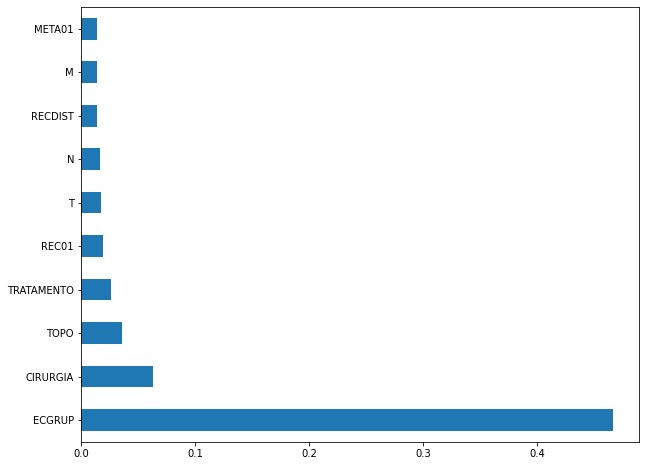
Here we noticed that the most used feature was
ECGRUP, with a good advantage. Following we haveCIRURGIA,TOPOandTRATAMENTO.
[ ]:
plot_shap_values(xgb_sp_12_15, X_testSP_12_15, feat_SP_12_15)
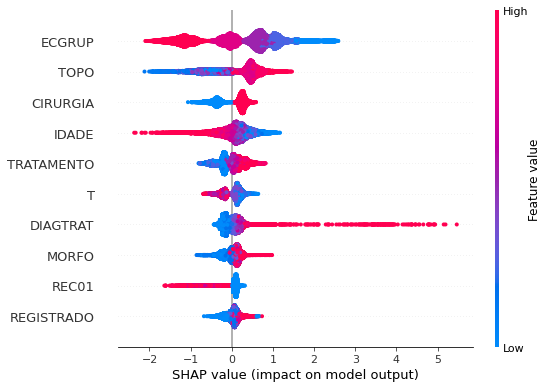
Note that larger values of the ECGRUP column, shown in pink, have more influence for the model’s prediction to be class 0, smaller values have greater weight for the prediction to be class 1. This behavior was expected, because the higher the clinical stage, worse is the stage of cancer.
The other columns shown follow the same logic.
[ ]:
# SP - 2016 to 2021
xgb_sp_16_21 = XGBClassifier(max_depth=8,
random_state=seed,
scale_pos_weight=1.28)
xgb_sp_16_21.fit(X_trainSP_16_21, y_trainSP_16_21)
XGBClassifier(max_depth=8, random_state=10, scale_pos_weight=1.28)
[ ]:
display_confusion_matrix(xgb_sp_16_21, X_testSP_16_21, y_testSP_16_21)

precision recall f1-score support
0 0.888 0.857 0.872 6773
1 0.821 0.859 0.840 5188
accuracy 0.858 11961
macro avg 0.855 0.858 0.856 11961
weighted avg 0.859 0.858 0.858 11961
The confusion matrix obtained for the XGBoost, with SP data from 2016 to 2021, shows a good performance of the model, with 86% of accuracy.
[ ]:
plot_roc_curve(xgb_sp_16_21, X_trainSP_16_21, X_testSP_16_21, y_trainSP_16_21, y_testSP_16_21)
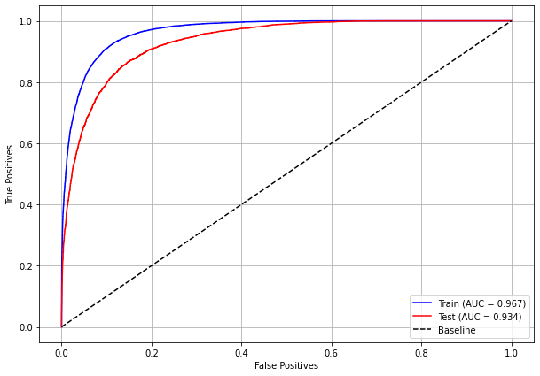
[ ]:
plot_feat_importances(xgb_sp_16_21, feat_SP_16_21)
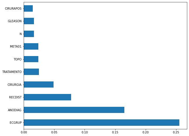
The four most important features were
ECGRUP,ANODIAG,RECDISTandCIRURGIA.
[ ]:
plot_shap_values(xgb_sp_16_21, X_testSP_16_21, feat_SP_16_21)
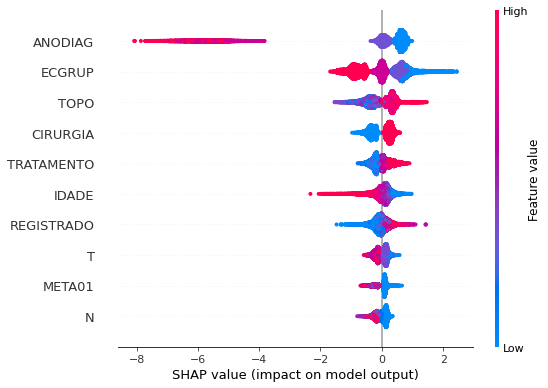
Note that larger values of the ANODIAG column, shown in pink, have more influence for the model’s prediction to be class 0, smaller values have greater weight for the prediction to be class 1.
The other columns shown follow the same logic.
Other states
[ ]:
# Other states - 2000 to 2003
xgb_fora_00_03 = XGBClassifier(max_depth=4,
scale_pos_weight=0.528,
random_state=seed)
xgb_fora_00_03.fit(X_trainOS_00_03, y_trainOS_00_03)
XGBClassifier(max_depth=4, random_state=10, scale_pos_weight=0.528)
[ ]:
display_confusion_matrix(xgb_fora_00_03, X_testOS_00_03, y_testOS_00_03)

precision recall f1-score support
0 0.705 0.783 0.742 351
1 0.844 0.781 0.811 526
accuracy 0.782 877
macro avg 0.775 0.782 0.777 877
weighted avg 0.788 0.782 0.784 877
The confusion matrix obtained for the XGBoost, with other states data from 2000 to 2003, also shows a good performance of the model, with 78% of accuracy.
[ ]:
plot_roc_curve(xgb_fora_00_03, X_trainOS_00_03, X_testOS_00_03, y_trainOS_00_03, y_testOS_00_03)
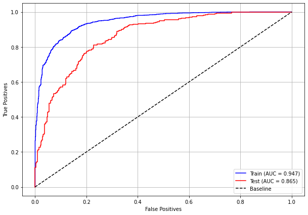
[ ]:
plot_feat_importances(xgb_fora_00_03, feat_OS_00_03)
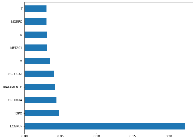
Again we noticed that the most used feature was
ECGRUP, with a good advantage. The following most important features wereTOPO,CIRURGIAandTRATAMENTO.
[ ]:
plot_shap_values(xgb_fora_00_03, X_testOS_00_03, feat_OS_00_03)
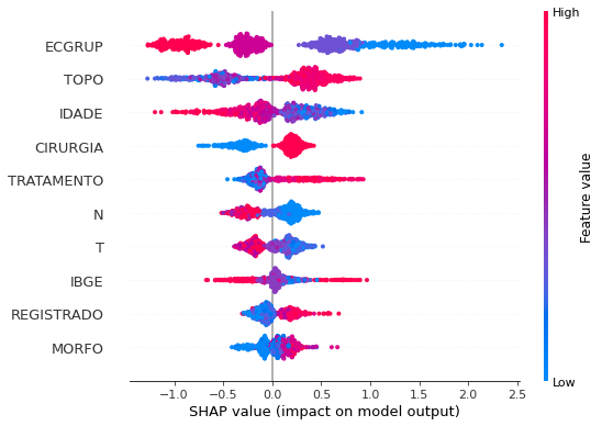
Note that larger values of the ECGRUP column, shown in pink, have more influence for the model’s prediction to be class 0, smaller values have greater weight for the prediction to be class 1. This behavior was expected, because the higher the clinical stage, worse is the stage of cancer.
The other columns shown follow the same logic.
[ ]:
# Other states - 2004 to 2007
xgb_fora_04_07 = XGBClassifier(max_depth=4,
scale_pos_weight=0.62,
random_state=seed)
xgb_fora_04_07.fit(X_trainOS_04_07, y_trainOS_04_07)
XGBClassifier(max_depth=4, random_state=10, scale_pos_weight=0.62)
[ ]:
display_confusion_matrix(xgb_fora_04_07, X_testOS_04_07, y_testOS_04_07)

precision recall f1-score support
0 0.708 0.808 0.754 443
1 0.881 0.809 0.843 775
accuracy 0.809 1218
macro avg 0.794 0.809 0.799 1218
weighted avg 0.818 0.809 0.811 1218
The confusion matrix obtained for the XGBoost, with other states data from 2004 to 2007, also shows a good performance of the model with 81% of accuracy.
[ ]:
plot_roc_curve(xgb_fora_04_07, X_trainOS_04_07, X_testOS_04_07, y_trainOS_04_07, y_testOS_04_07)
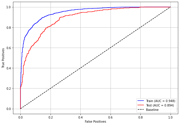
[ ]:
plot_feat_importances(xgb_fora_04_07, feat_OS_04_07)
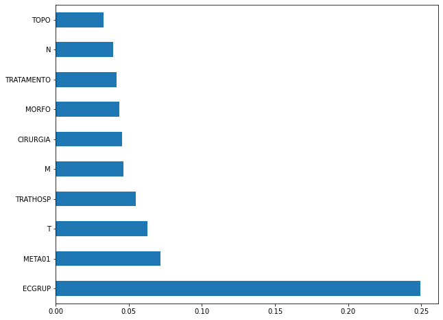
Again we noticed that the most used feature was
ECGRUP, with a good advantage. The following most important features wereMETA01,TandTRATHOSP.
[ ]:
plot_shap_values(xgb_fora_04_07, X_testOS_04_07, feat_OS_04_07)
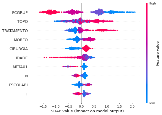
Note that larger values of the ECGRUP column, shown in pink, have more influence for the model’s prediction to be class 0, smaller values have greater weight for the prediction to be class 1. This behavior was expected, because the higher the clinical stage, worse is the stage of cancer.
The other columns shown follow the same logic.
[ ]:
# Other states - 2008 to 2011
xgb_fora_08_11 = XGBClassifier(max_depth=4,
scale_pos_weight=0.5,
random_state=seed)
xgb_fora_08_11.fit(X_trainOS_08_11, y_trainOS_08_11)
XGBClassifier(max_depth=4, random_state=10, scale_pos_weight=0.5)
[ ]:
display_confusion_matrix(xgb_fora_08_11, X_testOS_08_11, y_testOS_08_11)

precision recall f1-score support
0 0.711 0.822 0.763 510
1 0.896 0.822 0.857 953
accuracy 0.822 1463
macro avg 0.804 0.822 0.810 1463
weighted avg 0.832 0.822 0.824 1463
The confusion matrix obtained for the XGBoost, with other states data from 2008 to 2011, also shows a good performance of the model with 82% of accuracy.
[ ]:
plot_roc_curve(xgb_fora_08_11, X_trainOS_08_11, X_testOS_08_11, y_trainOS_08_11, y_testOS_08_11)
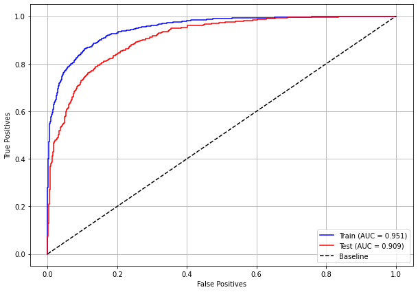
[ ]:
plot_feat_importances(xgb_fora_08_11, feat_OS_08_11)
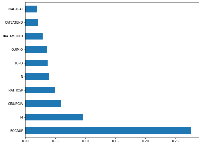
Again we noticed that the most used feature was
ECGRUP, but not with a lot of advantage. The following most important features wereM,CIRURGIAandTRATHOSP.
[ ]:
plot_shap_values(xgb_fora_08_11, X_testOS_08_11, feat_OS_08_11)
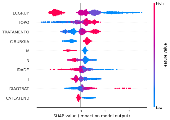
Note that larger values of the ECGRUP column, shown in pink, have more influence for the model’s prediction to be class 0, smaller values have greater weight for the prediction to be class 1. This behavior was expected, because the higher the clinical stage, worse is the stage of cancer.
The other columns shown follow the same logic.
[ ]:
# Other states - 2012 to 2015
xgb_fora_12_15 = XGBClassifier(max_depth=5,
scale_pos_weight=0.36,
random_state=seed)
xgb_fora_12_15.fit(X_trainOS_12_15, y_trainOS_12_15)
XGBClassifier(max_depth=5, random_state=10, scale_pos_weight=0.36)
[ ]:
display_confusion_matrix(xgb_fora_12_15, X_testOS_12_15, y_testOS_12_15)

precision recall f1-score support
0 0.693 0.827 0.754 571
1 0.910 0.827 0.867 1211
accuracy 0.827 1782
macro avg 0.802 0.827 0.810 1782
weighted avg 0.841 0.827 0.831 1782
The confusion matrix obtained for the XGBoost, with other states data from 2012 to 2015, also shows a good performance of the model with 83% of accuracy.
[ ]:
plot_roc_curve(xgb_fora_12_15, X_trainOS_12_15, X_testOS_12_15, y_trainOS_12_15, y_testOS_12_15)
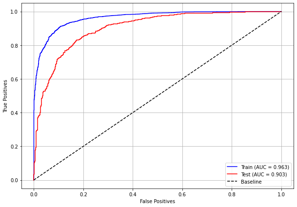
[ ]:
plot_feat_importances(xgb_fora_12_15, feat_OS_12_15)
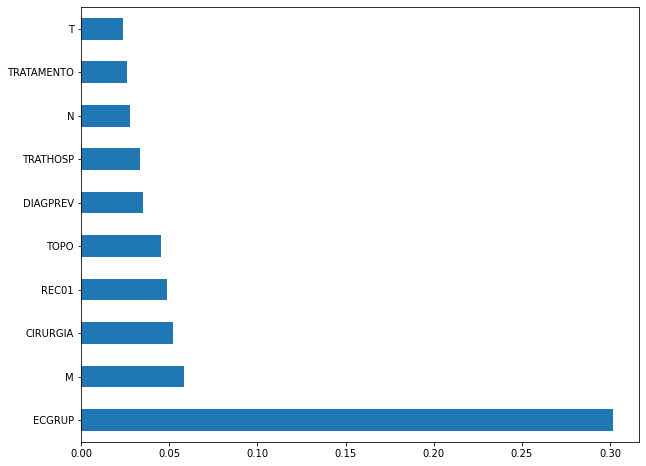
The four most important features were
ECGRUP,M,CIRURGIAandREC01.
[ ]:
plot_shap_values(xgb_fora_12_15, X_testOS_12_15, feat_OS_12_15)
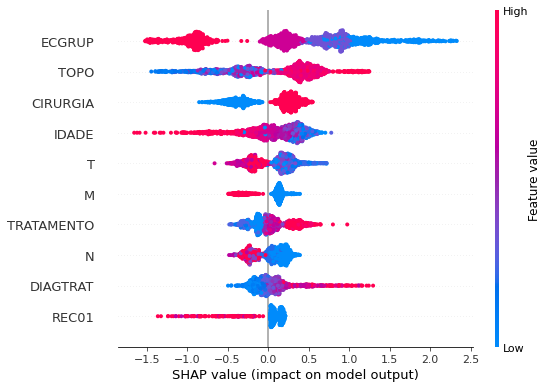
Note that larger values of the ECGRUP column, shown in pink, have more influence for the model’s prediction to be class 0, smaller values have greater weight for the prediction to be class 1. This behavior was expected, because the higher the clinical stage, worse is the stage of cancer.
The other columns shown follow the same logic.
[ ]:
# Other states - 2016 to 2020
xgb_fora_16_20 = XGBClassifier(max_depth=5,
scale_pos_weight=1.02,
random_state=seed)
xgb_fora_16_20.fit(X_trainOS_16_20, y_trainOS_16_20)
XGBClassifier(max_depth=5, random_state=10, scale_pos_weight=1.02)
[ ]:
display_confusion_matrix(xgb_fora_16_20, X_testOS_16_20, y_testOS_16_20)

precision recall f1-score support
0 0.878 0.857 0.868 539
1 0.831 0.855 0.843 442
accuracy 0.856 981
macro avg 0.855 0.856 0.855 981
weighted avg 0.857 0.856 0.856 981
The confusion matrix obtained for the XGBoost, with other states data from 2016 to 2020, shows the best performance comparing with the other models, with 86% of accuracy.
[ ]:
plot_roc_curve(xgb_fora_16_20, X_trainOS_16_20, X_testOS_16_20, y_trainOS_16_20, y_testOS_16_20)

[ ]:
plot_feat_importances(xgb_fora_16_20, feat_OS_16_20)
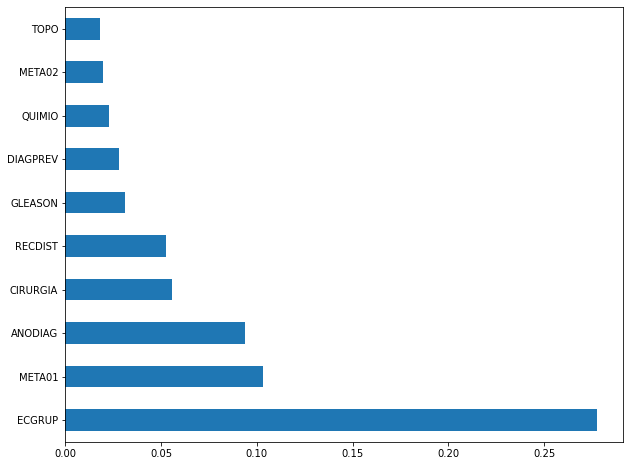
The four most important features were
ECGRUP,META01,ANODIAGandCIRURGIA.
[ ]:
plot_shap_values(xgb_fora_16_20, X_testOS_16_20, feat_OS_16_20)
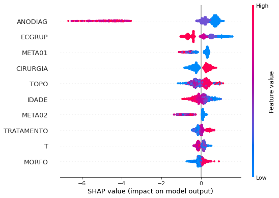
Note that larger values of the ANODIAG column, shown in pink, have more influence for the model’s prediction to be class 0, smaller values have greater weight for the prediction to be class 1.
The other columns shown follow the same logic.
Testing models with data from other years
We will use test data from the following years in the trained models for each set of years grouped together.
Random Forest SP for years 2000 to 2003
[ ]:
display_confusion_matrix(rf_sp_00_03, X_testSP_04_07, y_testSP_04_07)

precision recall f1-score support
0 0.728 0.788 0.757 7568
1 0.855 0.810 0.832 11699
accuracy 0.801 19267
macro avg 0.791 0.799 0.794 19267
weighted avg 0.805 0.801 0.802 19267
[ ]:
display_confusion_matrix(rf_sp_00_03, X_testSP_08_11, y_testSP_08_11)

precision recall f1-score support
0 0.711 0.769 0.739 9635
1 0.856 0.814 0.835 16251
accuracy 0.798 25886
macro avg 0.783 0.792 0.787 25886
weighted avg 0.802 0.798 0.799 25886
[ ]:
display_confusion_matrix(rf_sp_00_03, X_testSP_12_15, y_testSP_12_15)

precision recall f1-score support
0 0.688 0.781 0.732 10563
1 0.871 0.806 0.837 19291
accuracy 0.797 29854
macro avg 0.779 0.794 0.784 29854
weighted avg 0.806 0.797 0.800 29854
[ ]:
display_confusion_matrix(rf_sp_00_03, X_testSP_16_21, y_testSP_16_21)
precision recall f1-score support
0 0.831 0.776 0.803 6773
1 0.731 0.794 0.761 5188
accuracy 0.784 11961
macro avg 0.781 0.785 0.782 11961
weighted avg 0.788 0.784 0.785 11961
XGBoost SP for years 2000 to 2003
[ ]:
display_confusion_matrix(xgb_sp_00_03, X_testSP_04_07, y_testSP_04_07)
precision recall f1-score support
0 0.752 0.768 0.760 7568
1 0.848 0.836 0.842 11699
accuracy 0.810 19267
macro avg 0.800 0.802 0.801 19267
weighted avg 0.810 0.810 0.810 19267
[ ]:
display_confusion_matrix(xgb_sp_00_03, X_testSP_08_11, y_testSP_08_11)
precision recall f1-score support
0 0.737 0.744 0.741 9635
1 0.848 0.843 0.845 16251
accuracy 0.806 25886
macro avg 0.793 0.794 0.793 25886
weighted avg 0.807 0.806 0.806 25886
[ ]:
display_confusion_matrix(xgb_sp_00_03, X_testSP_12_15, y_testSP_12_15)

precision recall f1-score support
0 0.715 0.726 0.720 10563
1 0.849 0.841 0.845 19291
accuracy 0.801 29854
macro avg 0.782 0.784 0.783 29854
weighted avg 0.801 0.801 0.801 29854
[ ]:
display_confusion_matrix(xgb_sp_00_03, X_testSP_16_21, y_testSP_16_21)
precision recall f1-score support
0 0.836 0.726 0.777 6773
1 0.695 0.814 0.750 5188
accuracy 0.764 11961
macro avg 0.765 0.770 0.764 11961
weighted avg 0.775 0.764 0.765 11961
Random Forest SP for years 2004 to 2007
[ ]:
display_confusion_matrix(rf_sp_04_07, X_testSP_08_11, y_testSP_08_11)
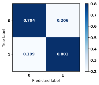
precision recall f1-score support
0 0.703 0.794 0.746 9635
1 0.868 0.801 0.833 16251
accuracy 0.798 25886
macro avg 0.785 0.797 0.789 25886
weighted avg 0.806 0.798 0.800 25886
[ ]:
display_confusion_matrix(rf_sp_04_07, X_testSP_12_15, y_testSP_12_15)

precision recall f1-score support
0 0.684 0.793 0.734 10563
1 0.876 0.800 0.836 19291
accuracy 0.797 29854
macro avg 0.780 0.796 0.785 29854
weighted avg 0.808 0.797 0.800 29854
[ ]:
display_confusion_matrix(rf_sp_04_07, X_testSP_16_21, y_testSP_16_21)

precision recall f1-score support
0 0.826 0.782 0.803 6773
1 0.734 0.784 0.758 5188
accuracy 0.783 11961
macro avg 0.780 0.783 0.781 11961
weighted avg 0.786 0.783 0.784 11961
XGBoost SP for years 2004 to 2007
[ ]:
display_confusion_matrix(xgb_sp_04_07, X_testSP_08_11, y_testSP_08_11)

precision recall f1-score support
0 0.735 0.778 0.756 9635
1 0.864 0.833 0.848 16251
accuracy 0.813 25886
macro avg 0.799 0.806 0.802 25886
weighted avg 0.816 0.813 0.814 25886
[ ]:
display_confusion_matrix(xgb_sp_04_07, X_testSP_12_15, y_testSP_12_15)

precision recall f1-score support
0 0.712 0.744 0.728 10563
1 0.856 0.835 0.846 19291
accuracy 0.803 29854
macro avg 0.784 0.790 0.787 29854
weighted avg 0.805 0.803 0.804 29854
[ ]:
display_confusion_matrix(xgb_sp_04_07, X_testSP_16_21, y_testSP_16_21)
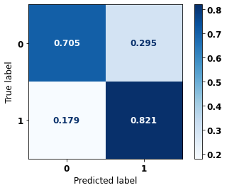
precision recall f1-score support
0 0.837 0.705 0.765 6773
1 0.681 0.821 0.744 5188
accuracy 0.755 11961
macro avg 0.759 0.763 0.755 11961
weighted avg 0.769 0.755 0.756 11961
Random Forest SP for years 2008 to 2011
[ ]:
display_confusion_matrix(rf_sp_08_11, X_testSP_12_15, y_testSP_12_15)
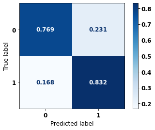
precision recall f1-score support
0 0.715 0.769 0.741 10563
1 0.868 0.832 0.850 19291
accuracy 0.810 29854
macro avg 0.792 0.801 0.796 29854
weighted avg 0.814 0.810 0.812 29854
[ ]:
display_confusion_matrix(rf_sp_08_11, X_testSP_16_21, y_testSP_16_21)
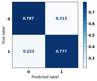
precision recall f1-score support
0 0.821 0.787 0.804 6773
1 0.736 0.777 0.756 5188
accuracy 0.782 11961
macro avg 0.779 0.782 0.780 11961
weighted avg 0.784 0.782 0.783 11961
XGBoost SP for years 2008 to 2011
[ ]:
display_confusion_matrix(xgb_sp_08_11, X_testSP_12_15, y_testSP_12_15)

precision recall f1-score support
0 0.756 0.692 0.722 10563
1 0.839 0.877 0.858 19291
accuracy 0.812 29854
macro avg 0.797 0.785 0.790 29854
weighted avg 0.809 0.812 0.810 29854
[ ]:
display_confusion_matrix(xgb_sp_08_11, X_testSP_16_21, y_testSP_16_21)
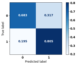
precision recall f1-score support
0 0.820 0.683 0.745 6773
1 0.660 0.805 0.725 5188
accuracy 0.735 11961
macro avg 0.740 0.744 0.735 11961
weighted avg 0.751 0.735 0.736 11961
Random Forest SP for years 2012 to 2015
[ ]:
display_confusion_matrix(rf_sp_12_15, X_testSP_16_21, y_testSP_16_21)

precision recall f1-score support
0 0.821 0.818 0.819 6773
1 0.763 0.767 0.765 5188
accuracy 0.796 11961
macro avg 0.792 0.792 0.792 11961
weighted avg 0.796 0.796 0.796 11961
XGBoost SP for years 2012 to 2015
[ ]:
display_confusion_matrix(xgb_sp_12_15, X_testSP_16_21, y_testSP_16_21)

precision recall f1-score support
0 0.814 0.828 0.821 6773
1 0.771 0.753 0.762 5188
accuracy 0.796 11961
macro avg 0.793 0.791 0.792 11961
weighted avg 0.795 0.796 0.796 11961
Random Forest Other states for years 2000 to 2003
[ ]:
display_confusion_matrix(rf_fora_00_03, X_testOS_04_07, y_testOS_04_07)
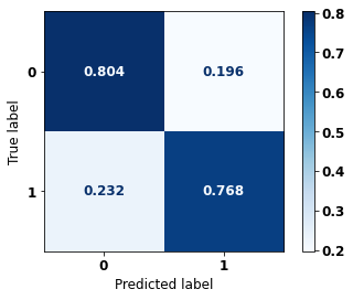
precision recall f1-score support
0 0.664 0.804 0.727 443
1 0.872 0.768 0.817 775
accuracy 0.781 1218
macro avg 0.768 0.786 0.772 1218
weighted avg 0.797 0.781 0.784 1218
[ ]:
display_confusion_matrix(rf_fora_00_03, X_testOS_08_11, y_testOS_08_11)

precision recall f1-score support
0 0.648 0.857 0.738 510
1 0.907 0.751 0.822 953
accuracy 0.788 1463
macro avg 0.778 0.804 0.780 1463
weighted avg 0.817 0.788 0.793 1463
[ ]:
display_confusion_matrix(rf_fora_00_03, X_testOS_12_15, y_testOS_12_15)

precision recall f1-score support
0 0.616 0.848 0.713 571
1 0.913 0.751 0.824 1211
accuracy 0.782 1782
macro avg 0.764 0.799 0.769 1782
weighted avg 0.818 0.782 0.788 1782
[ ]:
display_confusion_matrix(rf_fora_00_03, X_testOS_16_20, y_testOS_16_20)

precision recall f1-score support
0 0.808 0.835 0.821 539
1 0.790 0.758 0.774 442
accuracy 0.800 981
macro avg 0.799 0.796 0.797 981
weighted avg 0.800 0.800 0.800 981
XGBoost Other states for years 2000 to 2003
[ ]:
display_confusion_matrix(xgb_fora_00_03, X_testOS_04_07, y_testOS_04_07)

precision recall f1-score support
0 0.693 0.837 0.759 443
1 0.895 0.788 0.838 775
accuracy 0.806 1218
macro avg 0.794 0.813 0.798 1218
weighted avg 0.821 0.806 0.809 1218
[ ]:
display_confusion_matrix(xgb_fora_00_03, X_testOS_08_11, y_testOS_08_11)

precision recall f1-score support
0 0.651 0.845 0.735 510
1 0.901 0.758 0.823 953
accuracy 0.788 1463
macro avg 0.776 0.801 0.779 1463
weighted avg 0.814 0.788 0.793 1463
[ ]:
display_confusion_matrix(xgb_fora_00_03, X_testOS_12_15, y_testOS_12_15)

precision recall f1-score support
0 0.632 0.828 0.717 571
1 0.905 0.773 0.834 1211
accuracy 0.791 1782
macro avg 0.769 0.801 0.776 1782
weighted avg 0.818 0.791 0.796 1782
[ ]:
display_confusion_matrix(xgb_fora_00_03, X_testOS_16_20, y_testOS_16_20)
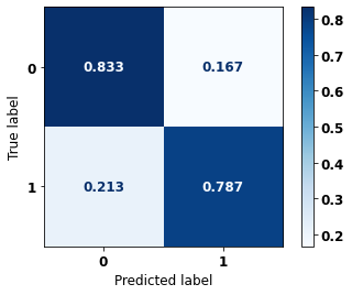
precision recall f1-score support
0 0.827 0.833 0.830 539
1 0.795 0.787 0.791 442
accuracy 0.812 981
macro avg 0.811 0.810 0.810 981
weighted avg 0.812 0.812 0.812 981
Random Forest Other states for years 2004 to 2007
[ ]:
display_confusion_matrix(rf_fora_04_07, X_testOS_08_11, y_testOS_08_11)

precision recall f1-score support
0 0.684 0.827 0.749 510
1 0.896 0.795 0.843 953
accuracy 0.807 1463
macro avg 0.790 0.811 0.796 1463
weighted avg 0.822 0.807 0.810 1463
[ ]:
display_confusion_matrix(rf_fora_04_07, X_testOS_12_15, y_testOS_12_15)
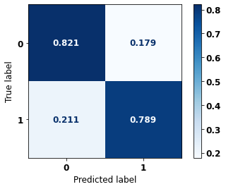
precision recall f1-score support
0 0.647 0.821 0.724 571
1 0.904 0.789 0.842 1211
accuracy 0.799 1782
macro avg 0.775 0.805 0.783 1782
weighted avg 0.821 0.799 0.804 1782
[ ]:
display_confusion_matrix(rf_fora_04_07, X_testOS_16_20, y_testOS_16_20)

precision recall f1-score support
0 0.818 0.833 0.825 539
1 0.792 0.774 0.783 442
accuracy 0.806 981
macro avg 0.805 0.803 0.804 981
weighted avg 0.806 0.806 0.806 981
XGBoost Other states for years 2004 to 2007
[ ]:
display_confusion_matrix(xgb_fora_04_07, X_testOS_08_11, y_testOS_08_11)

precision recall f1-score support
0 0.696 0.831 0.758 510
1 0.899 0.806 0.850 953
accuracy 0.815 1463
macro avg 0.798 0.819 0.804 1463
weighted avg 0.829 0.815 0.818 1463
[ ]:
display_confusion_matrix(xgb_fora_04_07, X_testOS_12_15, y_testOS_12_15)

precision recall f1-score support
0 0.649 0.811 0.721 571
1 0.899 0.794 0.843 1211
accuracy 0.799 1782
macro avg 0.774 0.802 0.782 1782
weighted avg 0.819 0.799 0.804 1782
[ ]:
display_confusion_matrix(xgb_fora_04_07, X_testOS_16_20, y_testOS_16_20)

precision recall f1-score support
0 0.827 0.833 0.830 539
1 0.795 0.787 0.791 442
accuracy 0.812 981
macro avg 0.811 0.810 0.810 981
weighted avg 0.812 0.812 0.812 981
Random Forest Other states for years 2008 to 2011
[ ]:
display_confusion_matrix(rf_fora_08_11, X_testOS_12_15, y_testOS_12_15)

precision recall f1-score support
0 0.666 0.793 0.724 571
1 0.893 0.813 0.851 1211
accuracy 0.806 1782
macro avg 0.780 0.803 0.788 1782
weighted avg 0.820 0.806 0.810 1782
[ ]:
display_confusion_matrix(rf_fora_08_11, X_testOS_16_20, y_testOS_16_20)
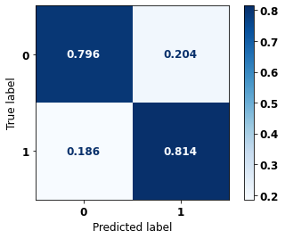
precision recall f1-score support
0 0.840 0.796 0.817 539
1 0.766 0.814 0.789 442
accuracy 0.804 981
macro avg 0.803 0.805 0.803 981
weighted avg 0.806 0.804 0.805 981
XGBoost Other states for years 2008 to 2011
[ ]:
display_confusion_matrix(xgb_fora_08_11, X_testOS_12_15, y_testOS_12_15)
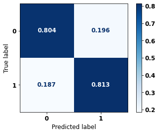
precision recall f1-score support
0 0.670 0.804 0.731 571
1 0.898 0.813 0.854 1211
accuracy 0.810 1782
macro avg 0.784 0.809 0.792 1782
weighted avg 0.825 0.810 0.814 1782
[ ]:
display_confusion_matrix(xgb_fora_08_11, X_testOS_16_20, y_testOS_16_20)

precision recall f1-score support
0 0.829 0.794 0.811 539
1 0.761 0.801 0.781 442
accuracy 0.797 981
macro avg 0.795 0.797 0.796 981
weighted avg 0.799 0.797 0.798 981
Random Forest Other states for years 2012 to 2015
[ ]:
display_confusion_matrix(rf_fora_12_15, X_testOS_16_20, y_testOS_16_20)

precision recall f1-score support
0 0.834 0.850 0.842 539
1 0.812 0.794 0.803 442
accuracy 0.825 981
macro avg 0.823 0.822 0.823 981
weighted avg 0.824 0.825 0.824 981
XGBoost Other states for years 2012 to 2015
[ ]:
display_confusion_matrix(xgb_fora_12_15, X_testOS_16_20, y_testOS_16_20)

precision recall f1-score support
0 0.833 0.853 0.843 539
1 0.816 0.792 0.804 442
accuracy 0.826 981
macro avg 0.825 0.823 0.823 981
weighted avg 0.825 0.826 0.825 981