Reading the data
Reading the raw data, these data have already been transformed into a csv file and the columns DTTRAT, DTULTINFO and DTRECIDIVA had the values #NULL! replaced by NaN.
[ ]:
data = read_csv('/content/drive/MyDrive/Trabalho/Cancer/Datasets/geral.csv')
data.head()
Columns (33,34,78,83,88,89,90) have mixed types.Specify dtype option on import or set low_memory=False.
(922473, 93)
| SEXO | IDADE | ESCOLARI | UFNASC | UFRESID | IBGE | CIDADE | CATEATEND | DTCONSULT | CLINICA | DIAGPREV | DTDIAG | BASEDIAG | TOPO | TOPOGRUP | DESCTOPO | MORFO | DESCMORFO | EC | ECGRUP | T | N | M | PT | PN | PM | S | G | LOCALTNM | IDMITOTIC | PSA | GLEASON | OUTRACLA | META01 | META02 | META03 | META04 | DTTRAT | NAOTRAT | TRATAMENTO | ... | RADIOANT | QUIMIOANT | HORMOANT | TMOANT | IMUNOANT | OUTROANT | NENHUMAPOS | CIRURAPOS | RADIOAPOS | QUIMIOAPOS | HORMOAPOS | TMOAPOS | IMUNOAPOS | OUTROAPOS | DTULTINFO | ULTINFO | CONSDIAG | TRATCONS | DIAGTRAT | ANODIAG | CICI | CICIGRUP | CICISUBGRU | FAIXAETAR | LATERALI | INSTORIG | DRS | RRAS | DTPREENCH | REGISTRADO | DTRECIDIVA | RECNENHUM | RECLOCAL | RECREGIO | RECDIST | REC01 | REC02 | REC03 | REC04 | HABILIT2 | |
|---|---|---|---|---|---|---|---|---|---|---|---|---|---|---|---|---|---|---|---|---|---|---|---|---|---|---|---|---|---|---|---|---|---|---|---|---|---|---|---|---|---|---|---|---|---|---|---|---|---|---|---|---|---|---|---|---|---|---|---|---|---|---|---|---|---|---|---|---|---|---|---|---|---|---|---|---|---|---|---|---|---|
| 0 | 1 | 41 | 2 | SP | SP | 3509502 | CAMPINAS | 9 | 2005-01-14 | 30 | 1 | 2005-06-30 | 3 | C179 | C17 | INTESTINO DELGADO SOE | 82611 | ADENOMA VILOSO SOE | Y | Y | Y | Y | Y | NaN | NaN | NaN | 8 | 8 | 8 | 8 | 8 | 8 | NaN | NaN | NaN | NaN | NaN | 2005-08-03 00:00:00 | 8 | F | ... | 0 | 0 | 0 | 0 | 0 | 0 | 1 | 0 | 0 | 0 | 0 | 0 | 0 | 0 | 2017-08-10 00:00:00 | 2.0 | 167 | 201.0 | 34.0 | 2005 | NaN | NaN | NaN | 40-49 | 8 | NaN | DRS 07 CAMPINAS | 15 | 2006-12-14 | 1.0 | NaN | 1 | 0 | 0 | 0 | NaN | NaN | NaN | NaN | 1 |
| 1 | 2 | 0 | 2 | SP | AM | 1302603 | MANAUS | 2 | 2012-05-23 | 25 | 2 | 2005-09-17 | 3 | C411 | C41 | MANDIBULA | 88231 | FIBROMA DESMOPLASICO | Y | Y | Y | Y | Y | NaN | NaN | NaN | 8 | 8 | 8 | 8 | 8 | 8 | NaN | NaN | NaN | NaN | NaN | 2012-05-23 00:00:00 | 8 | E | ... | 0 | 0 | 0 | 0 | 0 | 0 | 0 | 0 | 0 | 1 | 0 | 0 | 0 | 0 | 2012-05-30 00:00:00 | 1.0 | 2440 | 0.0 | 2440.0 | 2005 | NaN | NaN | NaN | 00-09 | 8 | NaN | NaN | 99 | 2015-01-08 | 1.0 | NaN | 1 | 0 | 0 | 0 | NaN | NaN | NaN | NaN | 2 |
| 2 | 1 | 56 | 9 | SP | SP | 3508702 | CACONDE | 9 | 2003-08-25 | 12 | 1 | 2003-08-26 | 3 | C186 | C18 | COLON DESCENDENTE | 82611 | ADENOMA VILOSO SOE | Y | Y | Y | Y | Y | NaN | NaN | NaN | 8 | 8 | 8 | 8 | 8 | 8 | NaN | NaN | NaN | NaN | NaN | 2003-10-15 00:00:00 | 8 | A | ... | 0 | 0 | 0 | 0 | 0 | 0 | 1 | 0 | 0 | 0 | 0 | 0 | 0 | 0 | 2003-11-26 00:00:00 | 3.0 | 1 | 51.0 | 50.0 | 2003 | NaN | NaN | NaN | 50-59 | 8 | NaN | DRS 14 SÃO JOÃO DA BOA VISTA | 15 | 2004-08-25 | 1.0 | NaN | 1 | 0 | 0 | 0 | NaN | NaN | NaN | NaN | 2 |
| 3 | 1 | 26 | 2 | MG | SP | 3529401 | MAUA | 9 | 2003-02-04 | 4 | 1 | 2003-05-29 | 3 | C491 | C49 | TEC CONJUNTIVOSUBCUTANEO E OUTROS TECIDOS MOLE... | 88231 | FIBROMA DESMOPLASICO | IIA | II | 2B | 0 | 0 | NaN | NaN | NaN | 8 | 1 | 8 | 8 | 8 | 8 | NaN | NaN | NaN | NaN | NaN | 2003-05-29 00:00:00 | 8 | I | ... | 0 | 0 | 0 | 0 | 0 | 0 | 1 | 0 | 0 | 0 | 0 | 0 | 0 | 0 | 2019-02-12 00:00:00 | 2.0 | 114 | 114.0 | 0.0 | 2003 | NaN | NaN | NaN | 20-29 | 8 | NaN | DRS 01 SÃO PAULO | 1 | 2003-12-01 | 1.0 | 2011-02-03 00:00:00 | 0 | 1 | 0 | 0 | C49 | NaN | NaN | NaN | 2 |
| 4 | 2 | 40 | 3 | BA | SP | 3550308 | SAO PAULO | 9 | 2000-08-29 | 3 | 2 | 2000-08-29 | 3 | C410 | C41 | OSSOS DO CRANIO E DA FACE E RESPECTIVAS ARTICU... | 88231 | FIBROMA DESMOPLASICO | Y | Y | Y | Y | Y | Y | Y | Y | 8 | 8 | 8 | 8 | 8 | 8 | NaN | NaN | NaN | NaN | NaN | 2001-02-12 00:00:00 | 8 | I | ... | 0 | 0 | 0 | 0 | 0 | 0 | 1 | 0 | 0 | 0 | 0 | 0 | 0 | 0 | 2002-04-24 00:00:00 | 3.0 | 0 | 167.0 | 167.0 | 2000 | NaN | NaN | NaN | 40-49 | 8 | NaN | DRS 01 SÃO PAULO | 6 | 2001-05-24 | 1.0 | 2001-09-15 00:00:00 | 1 | 0 | 0 | 0 | NaN | NaN | NaN | NaN | 1 |
5 rows × 93 columns
[ ]:
# #NULL! to NaN
# data.loc[data.DTRECIDIVA == '#NULL!', 'DTRECIDIVA'] = np.nan
# data.loc[data.DTTRAT == '#NULL!', 'DTTRAT'] = np.nan
# data.loc[data.DTULTINFO == '#NULL!', 'DTULTINFO'] = np.nan
[ ]:
# save_csv(data, '/content/drive/MyDrive/Trabalho/Cancer/Datasets/geral.csv')
Data analysis
In this section we will analyze some data information with graphs, missing values and each column of the dataset individually.
Information
To start we have the most basic information of the data, such as the size of the dataset, the first lines, type of each column and the describe function that brings some statistical information for each column.
[ ]:
data.shape
(922473, 93)
[ ]:
data.head()
| SEXO | IDADE | ESCOLARI | UFNASC | UFRESID | IBGE | CIDADE | CATEATEND | DTCONSULT | CLINICA | DIAGPREV | DTDIAG | BASEDIAG | TOPO | TOPOGRUP | DESCTOPO | MORFO | DESCMORFO | EC | ECGRUP | T | N | M | PT | PN | PM | S | G | LOCALTNM | IDMITOTIC | PSA | GLEASON | OUTRACLA | META01 | META02 | META03 | META04 | DTTRAT | NAOTRAT | TRATAMENTO | ... | RADIOANT | QUIMIOANT | HORMOANT | TMOANT | IMUNOANT | OUTROANT | NENHUMAPOS | CIRURAPOS | RADIOAPOS | QUIMIOAPOS | HORMOAPOS | TMOAPOS | IMUNOAPOS | OUTROAPOS | DTULTINFO | ULTINFO | CONSDIAG | TRATCONS | DIAGTRAT | ANODIAG | CICI | CICIGRUP | CICISUBGRU | FAIXAETAR | LATERALI | INSTORIG | DRS | RRAS | DTPREENCH | REGISTRADO | DTRECIDIVA | RECNENHUM | RECLOCAL | RECREGIO | RECDIST | REC01 | REC02 | REC03 | REC04 | HABILIT2 | |
|---|---|---|---|---|---|---|---|---|---|---|---|---|---|---|---|---|---|---|---|---|---|---|---|---|---|---|---|---|---|---|---|---|---|---|---|---|---|---|---|---|---|---|---|---|---|---|---|---|---|---|---|---|---|---|---|---|---|---|---|---|---|---|---|---|---|---|---|---|---|---|---|---|---|---|---|---|---|---|---|---|---|
| 0 | 1 | 41 | 2 | SP | SP | 3509502 | CAMPINAS | 9 | 2005-01-14 | 30 | 1 | 2005-06-30 | 3 | C179 | C17 | INTESTINO DELGADO SOE | 82611 | ADENOMA VILOSO SOE | Y | Y | Y | Y | Y | NaN | NaN | NaN | 8 | 8 | 8 | 8 | 8 | 8 | NaN | NaN | NaN | NaN | NaN | 2005-08-03 00:00:00 | 8 | F | ... | 0 | 0 | 0 | 0 | 0 | 0 | 1 | 0 | 0 | 0 | 0 | 0 | 0 | 0 | 2017-08-10 00:00:00 | 2.0 | 167 | 201.0 | 34.0 | 2005 | NaN | NaN | NaN | 40-49 | 8 | NaN | DRS 07 CAMPINAS | 15 | 2006-12-14 | 1.0 | NaN | 1 | 0 | 0 | 0 | NaN | NaN | NaN | NaN | 1 |
| 1 | 2 | 0 | 2 | SP | AM | 1302603 | MANAUS | 2 | 2012-05-23 | 25 | 2 | 2005-09-17 | 3 | C411 | C41 | MANDIBULA | 88231 | FIBROMA DESMOPLASICO | Y | Y | Y | Y | Y | NaN | NaN | NaN | 8 | 8 | 8 | 8 | 8 | 8 | NaN | NaN | NaN | NaN | NaN | 2012-05-23 00:00:00 | 8 | E | ... | 0 | 0 | 0 | 0 | 0 | 0 | 0 | 0 | 0 | 1 | 0 | 0 | 0 | 0 | 2012-05-30 00:00:00 | 1.0 | 2440 | 0.0 | 2440.0 | 2005 | NaN | NaN | NaN | 00-09 | 8 | NaN | NaN | 99 | 2015-01-08 | 1.0 | NaN | 1 | 0 | 0 | 0 | NaN | NaN | NaN | NaN | 2 |
| 2 | 1 | 56 | 9 | SP | SP | 3508702 | CACONDE | 9 | 2003-08-25 | 12 | 1 | 2003-08-26 | 3 | C186 | C18 | COLON DESCENDENTE | 82611 | ADENOMA VILOSO SOE | Y | Y | Y | Y | Y | NaN | NaN | NaN | 8 | 8 | 8 | 8 | 8 | 8 | NaN | NaN | NaN | NaN | NaN | 2003-10-15 00:00:00 | 8 | A | ... | 0 | 0 | 0 | 0 | 0 | 0 | 1 | 0 | 0 | 0 | 0 | 0 | 0 | 0 | 2003-11-26 00:00:00 | 3.0 | 1 | 51.0 | 50.0 | 2003 | NaN | NaN | NaN | 50-59 | 8 | NaN | DRS 14 SÃO JOÃO DA BOA VISTA | 15 | 2004-08-25 | 1.0 | NaN | 1 | 0 | 0 | 0 | NaN | NaN | NaN | NaN | 2 |
| 3 | 1 | 26 | 2 | MG | SP | 3529401 | MAUA | 9 | 2003-02-04 | 4 | 1 | 2003-05-29 | 3 | C491 | C49 | TEC CONJUNTIVOSUBCUTANEO E OUTROS TECIDOS MOLE... | 88231 | FIBROMA DESMOPLASICO | IIA | II | 2B | 0 | 0 | NaN | NaN | NaN | 8 | 1 | 8 | 8 | 8 | 8 | NaN | NaN | NaN | NaN | NaN | 2003-05-29 00:00:00 | 8 | I | ... | 0 | 0 | 0 | 0 | 0 | 0 | 1 | 0 | 0 | 0 | 0 | 0 | 0 | 0 | 2019-02-12 00:00:00 | 2.0 | 114 | 114.0 | 0.0 | 2003 | NaN | NaN | NaN | 20-29 | 8 | NaN | DRS 01 SÃO PAULO | 1 | 2003-12-01 | 1.0 | 2011-02-03 00:00:00 | 0 | 1 | 0 | 0 | C49 | NaN | NaN | NaN | 2 |
| 4 | 2 | 40 | 3 | BA | SP | 3550308 | SAO PAULO | 9 | 2000-08-29 | 3 | 2 | 2000-08-29 | 3 | C410 | C41 | OSSOS DO CRANIO E DA FACE E RESPECTIVAS ARTICU... | 88231 | FIBROMA DESMOPLASICO | Y | Y | Y | Y | Y | Y | Y | Y | 8 | 8 | 8 | 8 | 8 | 8 | NaN | NaN | NaN | NaN | NaN | 2001-02-12 00:00:00 | 8 | I | ... | 0 | 0 | 0 | 0 | 0 | 0 | 1 | 0 | 0 | 0 | 0 | 0 | 0 | 0 | 2002-04-24 00:00:00 | 3.0 | 0 | 167.0 | 167.0 | 2000 | NaN | NaN | NaN | 40-49 | 8 | NaN | DRS 01 SÃO PAULO | 6 | 2001-05-24 | 1.0 | 2001-09-15 00:00:00 | 1 | 0 | 0 | 0 | NaN | NaN | NaN | NaN | 1 |
5 rows × 93 columns
[ ]:
data.info()
<class 'pandas.core.frame.DataFrame'>
RangeIndex: 922473 entries, 0 to 922472
Data columns (total 93 columns):
 #   Column      Non-Null Count   Dtype
---  ------      --------------   -----
 0   SEXO        922473 non-null  int64
 1   IDADE       922473 non-null  int64
 2   ESCOLARI    922473 non-null  int64
 3   UFNASC      922473 non-null  object
 4   UFRESID     922473 non-null  object
 5   IBGE        922473 non-null  int64
 6   CIDADE      922473 non-null  object
 7   CATEATEND   922473 non-null  int64
 8   DTCONSULT   922473 non-null  object
 9   CLINICA     922473 non-null  int64
 10  DIAGPREV    922473 non-null  int64
 11  DTDIAG      922473 non-null  object
 12  BASEDIAG    922473 non-null  int64
 13  TOPO        922473 non-null  object
 14  TOPOGRUP    922473 non-null  object
 15  DESCTOPO    922473 non-null  object
 16  MORFO       922473 non-null  int64
 17  DESCMORFO   922469 non-null  object
 18  EC          922473 non-null  object
 19  ECGRUP      922473 non-null  object
 20  T           922473 non-null  object
 21  N           922473 non-null  object
 22  M           922473 non-null  object
 23  PT          410793 non-null  object
 24  PN          408776 non-null  object
 25  PM          393210 non-null  object
 26  S           922473 non-null  int64
 27  G           922473 non-null  int64
 28  LOCALTNM    922473 non-null  int64
 29  IDMITOTIC   922473 non-null  int64
 30  PSA         922473 non-null  int64
 31  GLEASON     922473 non-null  int64
 32  OUTRACLA    444 non-null     float64
 33  META01      123162 non-null  object
 34  META02      38201 non-null   object
 35  META03      0 non-null       float64
 36  META04      0 non-null       float64
 37  DTTRAT      848682 non-null  object
 38  NAOTRAT     922473 non-null  int64
 39  TRATAMENTO  922473 non-null  object
 40  TRATHOSP    922473 non-null  object
 41  TRATFANTES  922473 non-null  object
 42  TRATFAPOS   922473 non-null  object
 43  NENHUM      922473 non-null  int64
 44  CIRURGIA    922473 non-null  int64
 45  RADIO       922473 non-null  int64
 46  QUIMIO      922473 non-null  int64
 47  HORMONIO    922473 non-null  int64
 48  TMO         922473 non-null  int64
 49  IMUNO       922473 non-null  int64
 50  OUTROS      922473 non-null  int64
 51  NENHUMANT   922473 non-null  int64
 52  CIRURANT    922473 non-null  int64
 53  RADIOANT    922473 non-null  int64
 54  QUIMIOANT   922473 non-null  int64
 55  HORMOANT    922473 non-null  int64
 56  TMOANT      922473 non-null  int64
 57  IMUNOANT    922473 non-null  int64
 58  OUTROANT    922473 non-null  int64
 59  NENHUMAPOS  922473 non-null  int64
 60  CIRURAPOS   922473 non-null  int64
 61  RADIOAPOS   922473 non-null  int64
 62  QUIMIOAPOS  922473 non-null  int64
 63  HORMOAPOS   922473 non-null  int64
 64  TMOAPOS     922473 non-null  int64
 65  IMUNOAPOS   922473 non-null  int64
 66  OUTROAPOS   922473 non-null  int64
 67  DTULTINFO   922425 non-null  object
 68  ULTINFO     922470 non-null  float64
 69  CONSDIAG    922473 non-null  int64
 70  TRATCONS    848682 non-null  float64
 71  DIAGTRAT    848682 non-null  float64
 72  ANODIAG     922473 non-null  int64
 73  CICI        0 non-null       float64
 74  CICIGRUP    0 non-null       float64
 75  CICISUBGRU  0 non-null       float64
 76  FAIXAETAR   922473 non-null  object
 77  LATERALI    922473 non-null  int64
 78  INSTORIG    469 non-null     object
 79  DRS         855995 non-null  object
 80  RRAS        922473 non-null  int64
 81  DTPREENCH   922473 non-null  object
 82  REGISTRADO  920925 non-null  float64
 83  DTRECIDIVA  96344 non-null   object
 84  RECNENHUM   922473 non-null  int64
 85  RECLOCAL    922473 non-null  int64
 86  RECREGIO    922473 non-null  int64
 87  RECDIST     922473 non-null  int64
 88  REC01       60075 non-null   object
 89  REC02       17512 non-null   object
 90  REC03       5594 non-null    object
 91  REC04       0 non-null       float64
 92  HABILIT2    922473 non-null  int64
dtypes: float64(11), int64(49), object(33)
memory usage: 654.5+ MB
[ ]:
data.describe()
| SEXO | IDADE | ESCOLARI | IBGE | CATEATEND | CLINICA | DIAGPREV | BASEDIAG | MORFO | S | G | LOCALTNM | IDMITOTIC | PSA | GLEASON | OUTRACLA | META03 | META04 | NAOTRAT | NENHUM | CIRURGIA | RADIO | QUIMIO | HORMONIO | TMO | IMUNO | OUTROS | NENHUMANT | CIRURANT | RADIOANT | QUIMIOANT | HORMOANT | TMOANT | IMUNOANT | OUTROANT | NENHUMAPOS | CIRURAPOS | RADIOAPOS | QUIMIOAPOS | HORMOAPOS | TMOAPOS | IMUNOAPOS | OUTROAPOS | ULTINFO | CONSDIAG | TRATCONS | DIAGTRAT | ANODIAG | CICI | CICIGRUP | CICISUBGRU | LATERALI | RRAS | REGISTRADO | RECNENHUM | RECLOCAL | RECREGIO | RECDIST | REC04 | HABILIT2 | |
|---|---|---|---|---|---|---|---|---|---|---|---|---|---|---|---|---|---|---|---|---|---|---|---|---|---|---|---|---|---|---|---|---|---|---|---|---|---|---|---|---|---|---|---|---|---|---|---|---|---|---|---|---|---|---|---|---|---|---|---|---|
| count | 922473.000000 | 922473.000000 | 922473.000000 | 9.224730e+05 | 922473.000000 | 922473.000000 | 922473.000000 | 922473.000000 | 922473.000000 | 922473.0 | 922473.000000 | 922473.000000 | 922473.000000 | 922473.000000 | 922473.000000 | 4.440000e+02 | 0.0 | 0.0 | 922473.000000 | 922473.000000 | 922473.000000 | 922473.000000 | 922473.000000 | 922473.000000 | 922473.000000 | 922473.000000 | 922473.000000 | 922473.000000 | 922473.000000 | 922473.000000 | 922473.0 | 922473.0 | 922473.0 | 922473.0 | 922473.0 | 922473.000000 | 922473.000000 | 922473.000000 | 922473.000000 | 922473.000000 | 922473.000000 | 922473.000000 | 922473.000000 | 922470.000000 | 922473.000000 | 848682.000000 | 848682.000000 | 922473.000000 | 0.0 | 0.0 | 0.0 | 922473.000000 | 922473.000000 | 920925.000000 | 922473.000000 | 922473.000000 | 922473.000000 | 922473.000000 | 0.0 | 922473.000000 |
| mean | 1.501193 | 59.773823 | 4.318006 | 3.543215e+06 | 4.790818 | 21.530410 | 1.380487 | 2.987335 | 83644.849173 | 8.0 | 7.853138 | 7.978581 | 7.996965 | 7.789755 | 7.797894 | 5.183580e+07 | NaN | NaN | 7.791193 | 0.083701 | 0.617216 | 0.264324 | 0.358157 | 0.124532 | 0.003842 | 0.006696 | 0.061035 | 0.999318 | 0.000001 | 0.000001 | 0.0 | 0.0 | 0.0 | 0.0 | 0.0 | 0.953824 | 0.004385 | 0.029604 | 0.007096 | 0.002158 | 0.000222 | 0.000149 | 0.006587 | 2.453364 | 53.022836 | 69.518061 | 67.831754 | 2010.591575 | NaN | NaN | NaN | 6.870138 | 15.829553 | 11.271003 | 0.913001 | 0.042336 | 0.024433 | 0.025516 | NaN | 1.635959 |
| std | 0.499999 | 16.907895 | 2.939945 | 3.465128e+05 | 3.519881 | 12.624555 | 0.485507 | 0.226864 | 4607.811838 | 0.0 | 0.947325 | 0.375104 | 0.141827 | 1.160094 | 1.109859 | 1.091127e+09 | NaN | NaN | 0.909882 | 0.276939 | 0.486067 | 0.440973 | 0.479459 | 0.330187 | 0.061863 | 0.081556 | 0.239394 | 0.026104 | 0.001041 | 0.001041 | 0.0 | 0.0 | 0.0 | 0.0 | 0.0 | 0.209866 | 0.066074 | 0.169493 | 0.083939 | 0.046408 | 0.014906 | 0.012186 | 0.080890 | 0.860908 | 165.460615 | 147.149209 | 151.181450 | 5.384567 | NaN | NaN | NaN | 2.470771 | 23.514225 | 11.528516 | 0.281833 | 0.201355 | 0.154390 | 0.157687 | NaN | 0.481160 |
| min | 1.000000 | 0.000000 | 1.000000 | 1.100015e+06 | 1.000000 | 1.000000 | 1.000000 | 1.000000 | 80001.000000 | 8.0 | 1.000000 | 1.000000 | 1.000000 | 1.000000 | 1.000000 | 0.000000e+00 | NaN | NaN | 1.000000 | 0.000000 | 0.000000 | 0.000000 | 0.000000 | 0.000000 | 0.000000 | 0.000000 | 0.000000 | 0.000000 | 0.000000 | 0.000000 | 0.0 | 0.0 | 0.0 | 0.0 | 0.0 | 0.000000 | 0.000000 | 0.000000 | 0.000000 | 0.000000 | 0.000000 | 0.000000 | 0.000000 | 1.000000 | 0.000000 | 0.000000 | 0.000000 | 2000.000000 | NaN | NaN | NaN | 1.000000 | 1.000000 | 0.000000 | 0.000000 | 0.000000 | 0.000000 | 0.000000 | NaN | 1.000000 |
| 25% | 1.000000 | 51.000000 | 2.000000 | 3.517406e+06 | 2.000000 | 12.000000 | 1.000000 | 3.000000 | 80703.000000 | 8.0 | 8.000000 | 8.000000 | 8.000000 | 8.000000 | 8.000000 | 0.000000e+00 | NaN | NaN | 8.000000 | 0.000000 | 0.000000 | 0.000000 | 0.000000 | 0.000000 | 0.000000 | 0.000000 | 0.000000 | 1.000000 | 0.000000 | 0.000000 | 0.0 | 0.0 | 0.0 | 0.0 | 0.0 | 1.000000 | 0.000000 | 0.000000 | 0.000000 | 0.000000 | 0.000000 | 0.000000 | 0.000000 | 2.000000 | 4.000000 | 13.000000 | 0.000000 | 2006.000000 | NaN | NaN | NaN | 8.000000 | 6.000000 | 2.000000 | 1.000000 | 0.000000 | 0.000000 | 0.000000 | NaN | 1.000000 |
| 50% | 2.000000 | 62.000000 | 3.000000 | 3.539301e+06 | 2.000000 | 24.000000 | 1.000000 | 3.000000 | 81403.000000 | 8.0 | 8.000000 | 8.000000 | 8.000000 | 8.000000 | 8.000000 | 1.000000e+00 | NaN | NaN | 8.000000 | 0.000000 | 1.000000 | 0.000000 | 0.000000 | 0.000000 | 0.000000 | 0.000000 | 0.000000 | 1.000000 | 0.000000 | 0.000000 | 0.0 | 0.0 | 0.0 | 0.0 | 0.0 | 1.000000 | 0.000000 | 0.000000 | 0.000000 | 0.000000 | 0.000000 | 0.000000 | 0.000000 | 2.000000 | 22.000000 | 40.000000 | 34.000000 | 2011.000000 | NaN | NaN | NaN | 8.000000 | 10.000000 | 7.000000 | 1.000000 | 0.000000 | 0.000000 | 0.000000 | NaN | 2.000000 |
| 75% | 2.000000 | 72.000000 | 9.000000 | 3.550308e+06 | 9.000000 | 29.000000 | 2.000000 | 3.000000 | 85003.000000 | 8.0 | 8.000000 | 8.000000 | 8.000000 | 8.000000 | 8.000000 | 2.000000e+00 | NaN | NaN | 8.000000 | 0.000000 | 1.000000 | 1.000000 | 1.000000 | 0.000000 | 0.000000 | 0.000000 | 0.000000 | 1.000000 | 0.000000 | 0.000000 | 0.0 | 0.0 | 0.0 | 0.0 | 0.0 | 1.000000 | 0.000000 | 0.000000 | 0.000000 | 0.000000 | 0.000000 | 0.000000 | 0.000000 | 3.000000 | 54.000000 | 82.000000 | 87.000000 | 2015.000000 | NaN | NaN | NaN | 8.000000 | 13.000000 | 16.000000 | 1.000000 | 0.000000 | 0.000000 | 0.000000 | NaN | 2.000000 |
| max | 2.000000 | 113.000000 | 9.000000 | 9.999999e+06 | 9.000000 | 99.000000 | 2.000000 | 9.000000 | 99893.000000 | 8.0 | 9.000000 | 9.000000 | 9.000000 | 9.000000 | 9.000000 | 2.299151e+10 | NaN | NaN | 9.000000 | 1.000000 | 1.000000 | 1.000000 | 1.000000 | 1.000000 | 1.000000 | 1.000000 | 1.000000 | 1.000000 | 1.000000 | 1.000000 | 0.0 | 0.0 | 0.0 | 0.0 | 0.0 | 1.000000 | 1.000000 | 1.000000 | 1.000000 | 1.000000 | 1.000000 | 1.000000 | 1.000000 | 4.000000 | 6980.000000 | 7132.000000 | 6891.000000 | 2021.000000 | NaN | NaN | NaN | 8.000000 | 99.000000 | 99.000000 | 1.000000 | 1.000000 | 1.000000 | 1.000000 | NaN | 2.000000 |
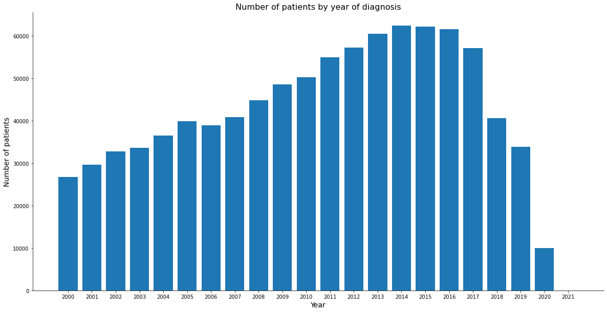
The first graph shows the number of patients per year of diagnosis, a low number of patients is perceived in recent years, probably due to the fact that these cases are still being followed up.
[ ]:
plt.figure(figsize=(20, 10))
plt.bar(height = data.ANODIAG.value_counts().sort_index(), x=np.sort(data.ANODIAG.unique()))
plt.xlabel('Year', size=14)
plt.xticks(np.sort(data.ANODIAG.unique()))
plt.ylabel('Number of patients', size=14)
plt.title('Number of patients by year of diagnosis', size=16)
plt.gca().spines['top'].set_visible(False)
plt.gca().spines['right'].set_visible(False)
plt.show()
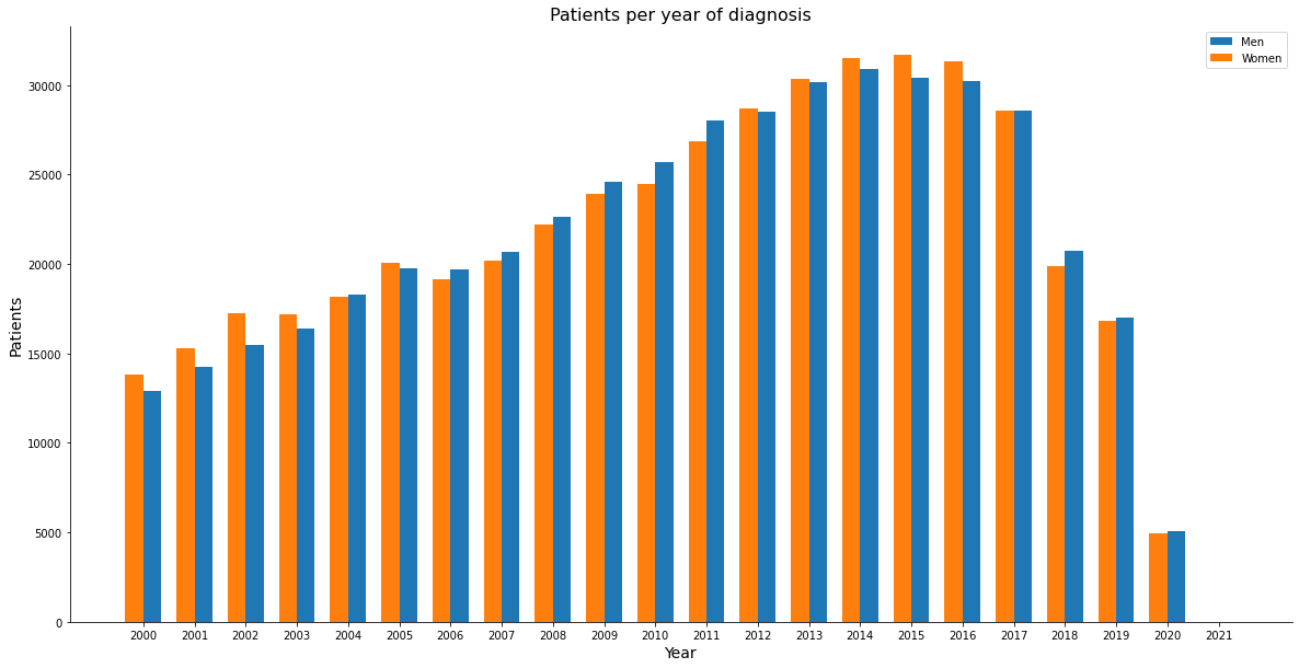
In the following graph we have the number of patients by sex, it’s possible to notice that in each year the values are close for men and women.
[ ]:
masc = data[data.SEXO == 1]
fem = data[data.SEXO == 2]

mascx = np.sort(masc.ANODIAG.unique())
mascy = masc.ANODIAG.value_counts().sort_index()

femx = np.sort(fem.ANODIAG.unique())
femy = fem.ANODIAG.value_counts().sort_index()
[ ]:
fig, ax = plt.subplots(figsize=(20, 10))
width = 0.35
ax1 = ax.bar(mascx + width/2, mascy, width, label='Men')
ax2 = ax.bar(femx - width/2, femy, width, label='Women')
ax.set_xlabel('Year', size=14)
ax.set_xticks(mascx)
ax.set_ylabel('Patients', size=14)
ax.set_title('Patients per year of diagnosis', size=16)

ax.legend()
ax.spines['top'].set_visible(False)
ax.spines['right'].set_visible(False)

plt.show()
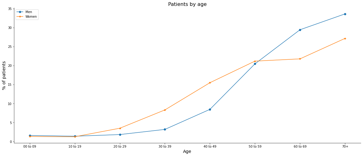
Analyzing the percentage of patients by age, we can see that women present the disease earlier, we have 23% of women from 30 to 49 years old against 11% of men in the same age group, but after 60 years old the number of men is higher in relation to women. It is also noticed that there is a higher incidence of cancer after 40 years old, with more than 85% of cases in both genders being in this age group.
[ ]:
# Using the replace to change the string format for the age group column
masc.FAIXAETAR = masc.FAIXAETAR.replace(['00-09', '10-19', '20-29', '30-39', '40-49', '50-59', '60-69'],
                                        ['00 to 09', '10 to 19', '20 to 29', '30 to 39', '40 to 49', '50 to 59', '60 to 69'])
fem.FAIXAETAR = fem.FAIXAETAR.replace(['00-09', '10-19', '20-29', '30-39', '40-49', '50-59', '60-69'],
                                      ['00 to 09', '10 to 19', '20 to 29', '30 to 39', '40 to 49', '50 to 59', '60 to 69'])
[ ]:
mascx = np.sort(masc.FAIXAETAR.unique())
mascy = masc.FAIXAETAR.value_counts().sort_index()

femx = np.sort(fem.FAIXAETAR.unique())
femy = fem.FAIXAETAR.value_counts().sort_index()
[ ]:
fig, ax = plt.subplots(figsize=(20, 8))
ax1 = ax.plot(mascx, (mascy/masc.shape[0])*100, label='Men', marker='o')
ax2 = ax.plot(femx, (femy/fem.shape[0])*100, label='Women', marker='*')
ax.set_xlabel('Age', size=14)
ax.set_ylabel('% of patients', size=14)
ax.set_title('Patients by age', size=16)

ax.legend()
ax.spines['top'].set_visible(False)
ax.spines['right'].set_visible(False)

plt.show()
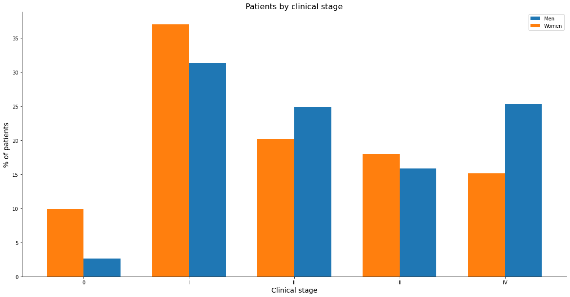
Looking at the clinical stage by sex, lower values for staging represent less aggressive diseases, we see women with more cases for stages 0, 1 and 3 and men with higher numbers in stage 2 and much higher in stage 4.
The clinical stage assists the doctors in the therapeutic planning and in the evaluation of the proposed treatment, in addition to serving for the prediction of the prognosis.
In the analysis of the data according to staging, cases reported as X (cases which it is not possible to perform staging or without information) and Y (type of cancer which the classification of malignant TNM tumors are not applied) were excluded.
[ ]:
EC = list(np.sort(data.ECGRUP.unique()))[:5] # Categories 0, I, II, III, IV, without X and Y

mascEC = masc.loc[masc.ECGRUP.isin(EC)]
femEC = fem.loc[fem.ECGRUP.isin(EC)]

mascx = np.sort(mascEC.ECGRUP.unique())
mascy = mascEC.ECGRUP.value_counts().sort_index()

femx = np.sort(femEC.ECGRUP.unique())
femy = femEC.ECGRUP.value_counts().sort_index()
[ ]:
x = np.arange(len(mascx))
fig, ax = plt.subplots(figsize=(20, 10))
width = 0.35
ax1 = ax.bar(x + width/2, (mascy/mascEC.shape[0])*100, width, label='Men')
ax2 = ax.bar(x - width/2, (femy/femEC.shape[0])*100, width, label='Women')
ax.set_xlabel('Clinical stage', size=14)
ax.set_ylabel('% of patients', size=14)
ax.set_title('Patients by clinical stage', size=16)

ax.legend()
ax.set_xticks(x)
ax.set_xticklabels(list(mascx))
ax.spines['top'].set_visible(False)
ax.spines['right'].set_visible(False)

plt.show()
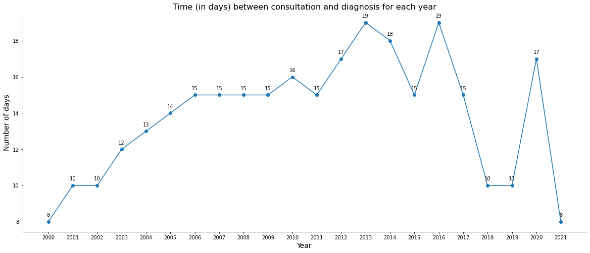
To analyze the time between consultation and diagnosis, the median number of days for each year was used, looking only at patients without diagnosis and without treatment in this first graph. For 2020 and 2021 we have less data, so the median is not realiable.
[ ]:
df_diag1 = data[data.DIAGPREV == 1] # without diagnosis/without treatment
df_diag2 = data[data.DIAGPREV == 2] # with diagnosis/without treatment
[ ]:
x = np.sort(df_diag1.ANODIAG.unique())
y = df_diag1.groupby('ANODIAG')['CONSDIAG'].median()
[ ]:
plt.figure(figsize=(20, 8))
plt.plot(x, y, marker='o')
plt.xlabel('Year', size=14)
plt.xticks(x)
plt.ylabel('Number of days', size=14)
plt.title('Time (in days) between consultation and diagnosis for each year', size=16)
for xi, yi in zip(x,y):
    label = '{:.0f}'.format(yi)
    plt.annotate(label, # this is the text
                 (xi, yi), # this is the point to label
                 textcoords='offset points', # how to position the text
                 xytext=(0, 10), # distance from text to points (x,y)
                 ha='center') # horizontal alignment can be left, right or center
plt.gca().spines['top'].set_visible(False)
plt.gca().spines['right'].set_visible(False)

plt.show()
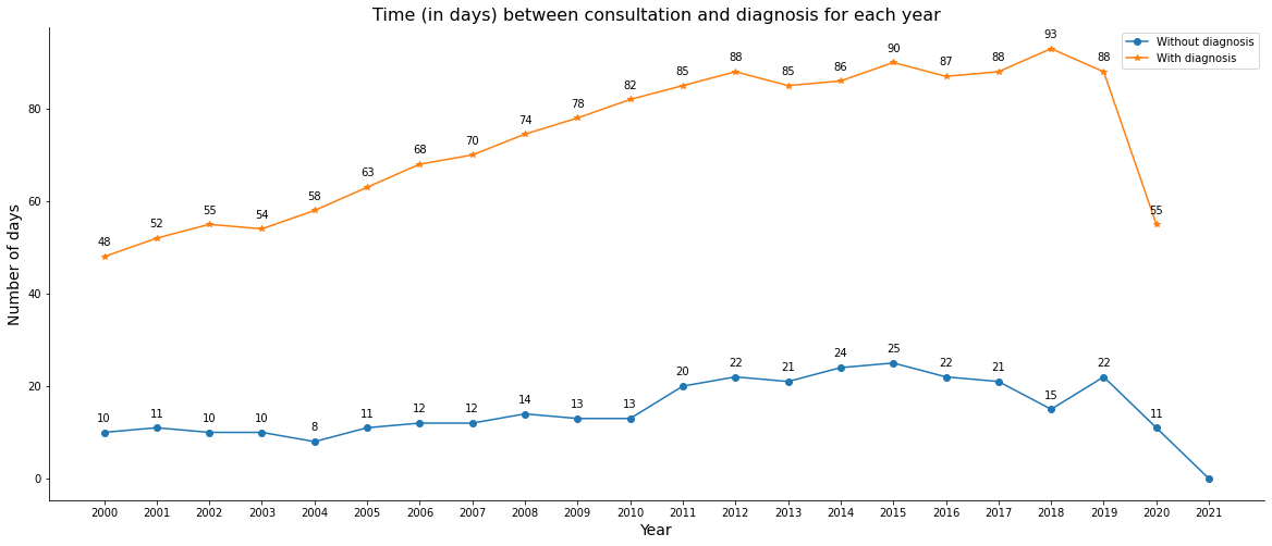
Now comparing patients without previous diagnosis with those who had the diagnosis, we can a much higher number of days to start treatment for people who already had the diagnosis of the disease, probably because they may have sought after other medical opinions, having gone to more than one hospital, delaying the start of cancer treatment.
In this analysis, C44 topographies (with morphologies between 80101 and 81103), who did not undergo any treatment (NAOTRAT = 8) and morphology 80001 (neoplasms with uncertain behavior) were excluded.
[ ]:
df1 = df_diag1[(df_diag1.TOPOGRUP == 'C44') & (df_diag1.MORFO > 80101) & (df_diag1.MORFO < 81103)]
df2 = df_diag2[(df_diag2.TOPOGRUP == 'C44') & (df_diag2.MORFO > 80101) & (df_diag2.MORFO < 81103)]

id1 = df1.index
df_diag1 = df_diag1.drop(id1)

id2 = df2.index
df_diag2 = df_diag2.drop(id2)

df_diag1 = df_diag1[(df_diag1.NAOTRAT == 8) & (df_diag1.MORFO != 80001)]
df_diag2 = df_diag2[(df_diag2.NAOTRAT == 8) & (df_diag2.MORFO != 80001)]

x1 = np.sort(df_diag1.ANODIAG.unique())
y1 = df_diag1.groupby('ANODIAG')['DIAGTRAT'].median()

x2 = np.sort(df_diag2.ANODIAG.unique())
y2 = df_diag2.groupby('ANODIAG')['DIAGTRAT'].median()
[ ]:
fig, ax = plt.subplots(figsize=(20, 8))
ax1 = ax.plot(x1, y1, label='Without diagnosis', marker='o')
ax2 = ax.plot(x2, y2, label='With diagnosis', marker='*')
ax.set_xlabel('Year', size=14)
ax.set_xticks(x1)
ax.set_ylabel('Number of days', size=14)
ax.set_title('Time (in days) between consultation and diagnosis for each year', size=16)
ax.legend()
for xi1, yi1, xi2, yi2 in zip(x1, y1, x2, y2):
    label1 = '{:.0f}'.format(yi1)
    label2 = '{:.0f}'.format(yi2)
    ax.annotate(label1, # this is the text
                (xi1, yi1), # this is the point to label
                textcoords='offset points', # how to position the text
                xytext=(0,10), # distance from text to points (x,y)
                ha='center') # horizontal alignment can be left, right or center
    ax.annotate(label2, # this is the text
                (xi2, yi2), # this is the point to label
                textcoords='offset points', # how to position the text
                xytext=(0,10), # distance from text to points (x,y)
                ha='center') # horizontal alignment can be left, right or center
ax.spines['top'].set_visible(False)
ax.spines['right'].set_visible(False)

plt.show()
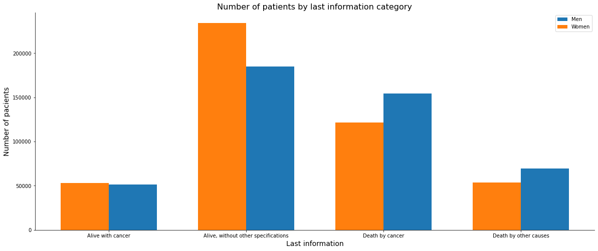
Now looking at the data from the latest patient information, we have a higher number of women in the category alive and of men in the two categories related to patient death, by cancer and other causes.
[ ]:
# 1 – Alive with cancer; 2 – Alive, without other specifications;
# 3 – Death by cancer; 4 – Death by other causes, without other specifications
data['ULTINFO'].value_counts()
2.0    419178
3.0    275748
4.0    123337
1.0    104207
Name: ULTINFO, dtype: int64
[ ]:
mascx = np.sort(masc.ULTINFO.unique())
mascy = masc.ULTINFO.value_counts().sort_index()

femx = np.sort(fem.ULTINFO.unique())
femy = fem.ULTINFO.value_counts().sort_index()

x_ticks = ['Alive with cancer', 'Alive, without other specifications', 'Death by cancer', 'Death by other causes']
[ ]:
x = np.arange(len(x_ticks))
fig, ax = plt.subplots(figsize=(20, 8))
width = 0.35
ax1 = ax.bar(x + width/2, mascy, width, label='Men')
ax2 = ax.bar(x - width/2, femy, width, label='Women')
ax.set_xlabel('Last information', size=14)
ax.set_ylabel('Number of pacients', size=14)
ax.set_title('Number of patients by last information category', size=16)

ax.legend()
ax.set_xticks(x)
ax.set_xticklabels(list(x_ticks))
ax.spines['top'].set_visible(False)
ax.spines['right'].set_visible(False)

plt.show()
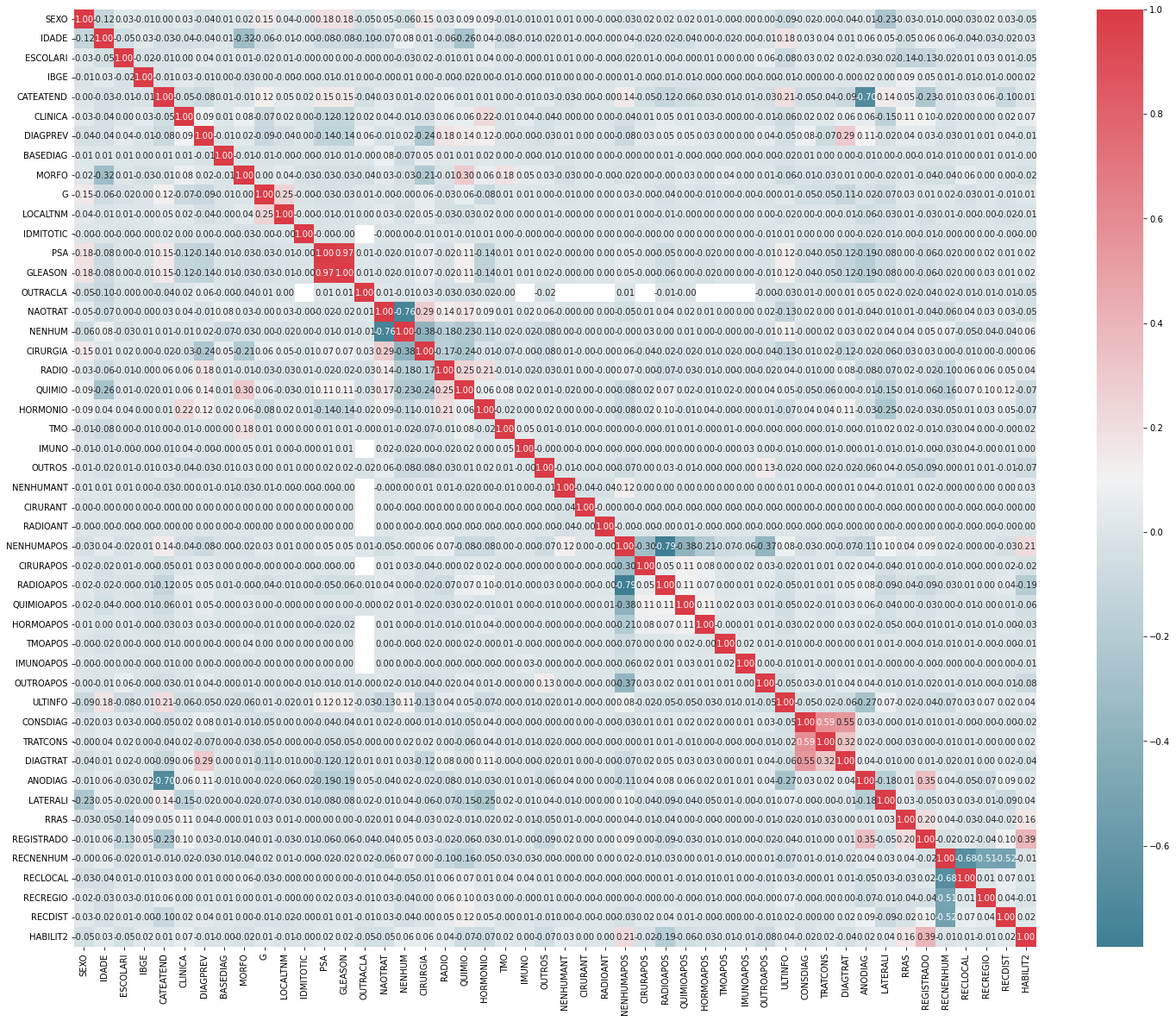
Now we will analyze the correlation of the ULTINFO column with the others in this dataset, we notice a good correlation with ANODIAG, which has the year of the patient’s diagnosis, and with CATEATEND, which indicates the category of patient care at the hospital, otherwise we don’t have such high correlations.
[ ]:
df_aux = data.copy()
df_aux.drop(columns=['S','META03','META04','QUIMIOANT','HORMOANT','TMOANT','IMUNOANT',
                     'OUTROANT','CICI','CICIGRUP','CICISUBGRU','REC04'], inplace=True)
corr_matrix = df_aux.corr()
abs(corr_matrix['ULTINFO']).sort_values(ascending = False)
ULTINFO       1.000000
ANODIAG       0.273169
CATEATEND     0.205837
IDADE         0.179007
CIRURGIA      0.128572
NAOTRAT       0.128528
GLEASON       0.118442
PSA           0.117614
NENHUM        0.112360
SEXO          0.085168
NENHUMAPOS    0.084783
ESCOLARI      0.077620
LATERALI      0.071756
RECREGIO      0.067356
RECNENHUM     0.066257
HORMONIO      0.065746
DIAGTRAT      0.059665
MORFO         0.059482
CLINICA       0.058677
OUTROAPOS     0.054789
QUIMIOAPOS    0.053917
QUIMIO        0.050139
CONSDIAG      0.050010
DIAGPREV      0.048716
RADIOAPOS     0.046268
HABILIT2      0.044645
REGISTRADO    0.036998
RADIO         0.036454
RECLOCAL      0.031626
HORMOAPOS     0.030271
OUTRACLA      0.029044
CIRURAPOS     0.024829
TRATCONS      0.023725
RRAS          0.022394
RECDIST       0.022101
LOCALTNM      0.020620
OUTROS        0.019981
BASEDIAG      0.017092
G             0.012019
IDMITOTIC     0.011892
IBGE          0.009061
NENHUMANT     0.008739
IMUNOAPOS     0.007141
IMUNO         0.006383
TMOAPOS       0.005317
TMO           0.004248
RADIOANT      0.000548
CIRURANT      0.000548
Name: ULTINFO, dtype: float64
In the correlation matrix we can see the correlations between all columns and as described above for the case of the analysis only for ULTINFO, we do not have very high correlations.
It is important to note that the data has not been processed yet, so after preprocessing a more explanatory matrix for the data can be obtained.
[ ]:
fig, ax = plt.subplots(figsize = (25, 20))
colormap = sns.diverging_palette(220, 10, as_cmap = True)

sns.heatmap(corr_matrix, cmap = colormap, annot = True, fmt = '.2f')
fig.show()
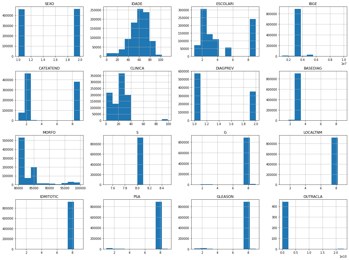
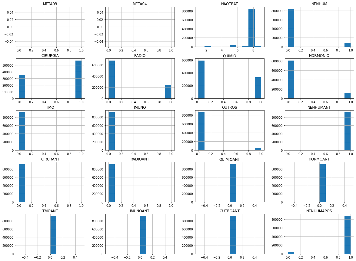
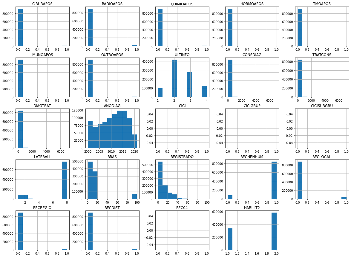
With the histograms you can see how the distributions of the dataset columns are, but since we have most of them with categorical data, the histograms bring information about the amount of data in the respective categories.
[ ]:
data.iloc[:,:35].hist(bins=10,figsize=(20, 15))
plt.show()
[ ]:
data.iloc[:,35:60].hist(bins=10,figsize=(20, 15))
plt.show()
[ ]:
data.iloc[:,60:].hist(bins=10,figsize=(20, 15))
plt.show()
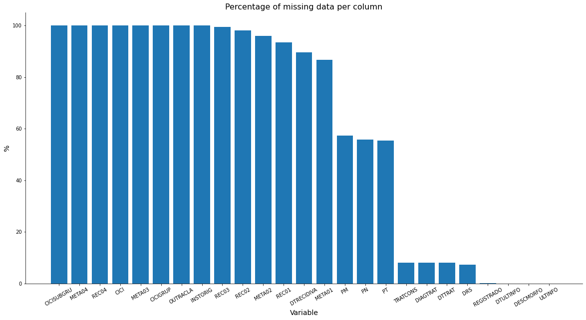
Missing values
Now let’s see the amount of missing values per column, we have 17 columns with more than 50% of missing data, being 6 with all missing values, if we want to use any of these for the machine learning models, it will be necessary to treat the missing values, placing 0 or some string that indicates that the value is missing, for example.
Another option is not using the columns in the analysis, we will see later in this project the proposed solutions to solve this problem.
[ ]:
missing = data.isna().sum().sort_values(ascending=False)
prop = missing[missing > 0]/data.shape[0]
prop
CICISUBGRU    1.000000
META04        1.000000
REC04         1.000000
CICI          1.000000
META03        1.000000
CICIGRUP      1.000000
OUTRACLA      0.999519
INSTORIG      0.999492
REC03         0.993936
REC02         0.981016
META02        0.958588
REC01         0.934876
DTRECIDIVA    0.895559
META01        0.866487
PM            0.573744
PN            0.556869
PT            0.554683
TRATCONS      0.079993
DIAGTRAT      0.079993
DTTRAT        0.079993
DRS           0.072065
REGISTRADO    0.001678
DTULTINFO     0.000052
DESCMORFO     0.000004
ULTINFO       0.000003
dtype: float64
[ ]:
plt.figure(figsize=(20, 10))
plt.bar(height = prop*100, x=prop.index)
plt.xlabel('Variable', size=14)
plt.ylabel('%', size=14)
plt.title('Percentage of missing data per column', size=16)
plt.xticks(rotation=30)
plt.gca().spines['top'].set_visible(False)
plt.gca().spines['right'].set_visible(False)
plt.show()
Columns analysis
In this section, the columns will be analyzed individually, with the aim of examining each one of them and obtaining a function that will be used in the data before starting the study with the machine learning models.
The columns were divided according to the type of each one, resulting in the categories: dates, numeric categories, letters categories, numbers, strings, letters and numbers categories.
Columns with unique values will be dropped from the dataset in the function called variables_preprocessing. Another treatment that will be done in the columns is the filling of string columns with missing values with ** Sem informação **, being the columns:
META01;META02;REC01;REC02;REC03;PT;PN;PM.
The DRS column will have the missing values filled with 0, after using the split method to obtain only the numbers in this column.
We also excluded from the data ECGRUP with X and Y values and C44 topographies (with morphologies between 80101 and 81103).
Finally, the columns that were dropped from the dataset, because they have unique values, only NaN values or because they are descriptions of the disease, are the following:
S;QUIMIOANT;HORMOANT;TMOANT;IMUNOANT;OUTROANT;UFNASC;CIDADE;DESCTOPO;DESCMORFO;CICISUBGRU;CICIGRUP;CICI;META03;META04;REC04;INSTORIG;OUTRACLA.
Check the functions section to see the complete function.
[ ]:
df_aux = read_csv('/content/drive/MyDrive/Trabalho/Cancer/Datasets/geral.csv')
Columns (33,34,78,83,88,89,90) have mixed types.Specify dtype option on import or set low_memory=False.
(922473, 93)
First preprocessing
Here the variables_preprocessing function will be applied, obtaining a new dataset with 75 columns (the raw data has 93 columns). It appears that we still have columns with missing values (DTRECIDIVA, TRATCONS, DTTRAT, DIAGTRAT, REGISTRADO and ULTINFO), all will be dealt with later.
After the function, the new dataset will be saved as a csv file, to be used in the sequence.
[ ]:
df = variables_preprocessing(df_aux)
df.head(3)
| SEXO | IDADE | ESCOLARI | UFRESID | IBGE | CATEATEND | DTCONSULT | CLINICA | DIAGPREV | DTDIAG | BASEDIAG | TOPO | TOPOGRUP | MORFO | EC | ECGRUP | T | N | M | PT | PN | PM | G | LOCALTNM | IDMITOTIC | PSA | GLEASON | META01 | META02 | DTTRAT | NAOTRAT | TRATAMENTO | TRATHOSP | TRATFANTES | TRATFAPOS | NENHUM | CIRURGIA | RADIO | QUIMIO | HORMONIO | TMO | IMUNO | OUTROS | NENHUMANT | CIRURANT | RADIOANT | NENHUMAPOS | CIRURAPOS | RADIOAPOS | QUIMIOAPOS | HORMOAPOS | TMOAPOS | IMUNOAPOS | OUTROAPOS | DTULTINFO | ULTINFO | CONSDIAG | TRATCONS | DIAGTRAT | ANODIAG | FAIXAETAR | LATERALI | DRS | RRAS | DTPREENCH | REGISTRADO | DTRECIDIVA | RECNENHUM | RECLOCAL | RECREGIO | RECDIST | REC01 | REC02 | REC03 | HABILIT2 | |
|---|---|---|---|---|---|---|---|---|---|---|---|---|---|---|---|---|---|---|---|---|---|---|---|---|---|---|---|---|---|---|---|---|---|---|---|---|---|---|---|---|---|---|---|---|---|---|---|---|---|---|---|---|---|---|---|---|---|---|---|---|---|---|---|---|---|---|---|---|---|---|---|---|---|---|---|
| 3 | 1 | 26 | 2 | SP | 3529401 | 9 | 2003-02-04 | 4 | 1 | 2003-05-29 | 3 | C491 | C49 | 88231 | IIA | II | 2B | 0 | 0 | **Sem informação** | **Sem informação** | **Sem informação** | 1 | 8 | 8 | 8 | 8 | **Sem informação** | **Sem informação** | 2003-05-29 00:00:00 | 8 | I | I | J | J | 0 | 1 | 1 | 0 | 1 | 0 | 0 | 0 | 1 | 0 | 0 | 1 | 0 | 0 | 0 | 0 | 0 | 0 | 0 | 2019-02-12 00:00:00 | 2.0 | 114 | 114.0 | 0.0 | 2003 | 20-29 | 8 | 01 | 1 | 2003-12-01 | 1.0 | 2011-02-03 00:00:00 | 0 | 1 | 0 | 0 | C49 | **Sem informação** | **Sem informação** | 2 |
| 29 | 1 | 50 | 9 | SP | 3531209 | 2 | 2016-01-15 | 26 | 2 | 2015-12-08 | 3 | C402 | C40 | 92613 | IA | I | 1 | 0 | 0 | 1 | 0 | 0 | 8 | 8 | 8 | 8 | 8 | **Sem informação** | **Sem informação** | 2016-02-29 00:00:00 | 8 | A | A | J | J | 0 | 1 | 0 | 0 | 0 | 0 | 0 | 0 | 1 | 0 | 0 | 1 | 0 | 0 | 0 | 0 | 0 | 0 | 0 | 2019-07-31 00:00:00 | 2.0 | 38 | 45.0 | 83.0 | 2015 | 50-59 | 8 | 07 | 15 | 2017-06-09 | 3.0 | NaN | 1 | 0 | 0 | 0 | **Sem informação** | **Sem informação** | **Sem informação** | 2 |
| 30 | 1 | 23 | 9 | SP | 3542602 | 9 | 2001-07-10 | 26 | 1 | 2001-10-29 | 3 | C402 | C40 | 92613 | IIB | II | 2 | 0 | 0 | 2 | 0 | 0 | 8 | 8 | 8 | 8 | 8 | **Sem informação** | **Sem informação** | 2001-10-29 00:00:00 | 8 | I | I | J | J | 0 | 1 | 0 | 0 | 0 | 0 | 0 | 1 | 1 | 0 | 0 | 1 | 0 | 0 | 0 | 0 | 0 | 0 | 0 | 2007-02-22 00:00:00 | 3.0 | 111 | 111.0 | 0.0 | 2001 | 20-29 | 8 | 12 | 7 | 2002-05-24 | 2.0 | 2004-06-22 00:00:00 | 0 | 0 | 1 | 0 | C34 | **Sem informação** | **Sem informação** | 1 |
[ ]:
df.shape
(581753, 75)
[ ]:
df.isna().sum().sort_values(ascending=False).head(8)
DTRECIDIVA    502783
DTTRAT         42795
TRATCONS       42795
DIAGTRAT       42795
DTULTINFO         30
ULTINFO            2
LOCALTNM           0
M                  0
dtype: int64
[ ]:
df.NAOTRAT.value_counts()
8    538811
5     18809
7      9862
2      7343
9      2615
6      1233
3      1123
4      1028
1       929
Name: NAOTRAT, dtype: int64
[ ]:
save_csv(df, '/content/drive/MyDrive/Trabalho/Cancer/Datasets/geral_pp.csv')
CSV file saved successfully!
Creating new columns
In this section, new columns will be created based on the difference between the date columns, the last information column and the recurrence column.
In addition, from here we will have two datasets, one with UFRESID for the São Paulo state and another one for the other states.
[ ]:
df = read_csv('/content/drive/MyDrive/Trabalho/Cancer/Datasets/geral_pp.csv')
df.head()
(581753, 75)
| SEXO | IDADE | ESCOLARI | UFRESID | IBGE | CATEATEND | DTCONSULT | CLINICA | DIAGPREV | DTDIAG | BASEDIAG | TOPO | TOPOGRUP | MORFO | EC | ECGRUP | T | N | M | PT | PN | PM | G | LOCALTNM | IDMITOTIC | PSA | GLEASON | META01 | META02 | DTTRAT | NAOTRAT | TRATAMENTO | TRATHOSP | TRATFANTES | TRATFAPOS | NENHUM | CIRURGIA | RADIO | QUIMIO | HORMONIO | TMO | IMUNO | OUTROS | NENHUMANT | CIRURANT | RADIOANT | NENHUMAPOS | CIRURAPOS | RADIOAPOS | QUIMIOAPOS | HORMOAPOS | TMOAPOS | IMUNOAPOS | OUTROAPOS | DTULTINFO | ULTINFO | CONSDIAG | TRATCONS | DIAGTRAT | ANODIAG | FAIXAETAR | LATERALI | DRS | RRAS | DTPREENCH | REGISTRADO | DTRECIDIVA | RECNENHUM | RECLOCAL | RECREGIO | RECDIST | REC01 | REC02 | REC03 | HABILIT2 | |
|---|---|---|---|---|---|---|---|---|---|---|---|---|---|---|---|---|---|---|---|---|---|---|---|---|---|---|---|---|---|---|---|---|---|---|---|---|---|---|---|---|---|---|---|---|---|---|---|---|---|---|---|---|---|---|---|---|---|---|---|---|---|---|---|---|---|---|---|---|---|---|---|---|---|---|---|
| 0 | 1 | 26 | 2 | SP | 3529401 | 9 | 2003-02-04 | 4 | 1 | 2003-05-29 | 3 | C491 | C49 | 88231 | IIA | II | 2B | 0 | 0 | **Sem informação** | **Sem informação** | **Sem informação** | 1 | 8 | 8 | 8 | 8 | **Sem informação** | **Sem informação** | 2003-05-29 00:00:00 | 8 | I | I | J | J | 0 | 1 | 1 | 0 | 1 | 0 | 0 | 0 | 1 | 0 | 0 | 1 | 0 | 0 | 0 | 0 | 0 | 0 | 0 | 2019-02-12 00:00:00 | 2.0 | 114 | 114.0 | 0.0 | 2003 | 20-29 | 8 | 1 | 1 | 2003-12-01 | 1.0 | 2011-02-03 00:00:00 | 0 | 1 | 0 | 0 | C49 | **Sem informação** | **Sem informação** | 2 |
| 1 | 1 | 50 | 9 | SP | 3531209 | 2 | 2016-01-15 | 26 | 2 | 2015-12-08 | 3 | C402 | C40 | 92613 | IA | I | 1 | 0 | 0 | 1 | 0 | 0 | 8 | 8 | 8 | 8 | 8 | **Sem informação** | **Sem informação** | 2016-02-29 00:00:00 | 8 | A | A | J | J | 0 | 1 | 0 | 0 | 0 | 0 | 0 | 0 | 1 | 0 | 0 | 1 | 0 | 0 | 0 | 0 | 0 | 0 | 0 | 2019-07-31 00:00:00 | 2.0 | 38 | 45.0 | 83.0 | 2015 | 50-59 | 8 | 7 | 15 | 2017-06-09 | 3.0 | NaN | 1 | 0 | 0 | 0 | **Sem informação** | **Sem informação** | **Sem informação** | 2 |
| 2 | 1 | 23 | 9 | SP | 3542602 | 9 | 2001-07-10 | 26 | 1 | 2001-10-29 | 3 | C402 | C40 | 92613 | IIB | II | 2 | 0 | 0 | 2 | 0 | 0 | 8 | 8 | 8 | 8 | 8 | **Sem informação** | **Sem informação** | 2001-10-29 00:00:00 | 8 | I | I | J | J | 0 | 1 | 0 | 0 | 0 | 0 | 0 | 1 | 1 | 0 | 0 | 1 | 0 | 0 | 0 | 0 | 0 | 0 | 0 | 2007-02-22 00:00:00 | 3.0 | 111 | 111.0 | 0.0 | 2001 | 20-29 | 8 | 12 | 7 | 2002-05-24 | 2.0 | 2004-06-22 00:00:00 | 0 | 0 | 1 | 0 | C34 | **Sem informação** | **Sem informação** | 1 |
| 3 | 2 | 14 | 9 | SP | 3518800 | 9 | 2006-08-15 | 26 | 1 | 2006-10-20 | 3 | C402 | C40 | 92613 | IB | I | 2 | 0 | 0 | 1 | 0 | 0 | 8 | 8 | 8 | 8 | 8 | **Sem informação** | **Sem informação** | 2006-10-20 00:00:00 | 8 | A | A | J | J | 0 | 1 | 0 | 0 | 0 | 0 | 0 | 0 | 1 | 0 | 0 | 1 | 0 | 0 | 0 | 0 | 0 | 0 | 0 | 2010-11-27 00:00:00 | 2.0 | 66 | 66.0 | 0.0 | 2006 | 10-19 | 8 | 1 | 2 | 2007-05-07 | 3.0 | NaN | 1 | 0 | 0 | 0 | **Sem informação** | **Sem informação** | **Sem informação** | 1 |
| 4 | 1 | 26 | 4 | AC | 1200401 | 2 | 2018-08-23 | 24 | 2 | 2018-07-13 | 3 | C402 | C40 | 92613 | IVA | IV | X | X | 1 | **Sem informação** | **Sem informação** | **Sem informação** | 8 | 8 | 8 | 8 | 8 | C34 | **Sem informação** | 2018-11-06 00:00:00 | 8 | A | A | J | J | 0 | 1 | 0 | 0 | 0 | 0 | 0 | 0 | 1 | 0 | 0 | 1 | 0 | 0 | 0 | 0 | 0 | 0 | 0 | 2020-06-22 00:00:00 | 1.0 | 41 | 75.0 | 116.0 | 2018 | 20-29 | 8 | 0 | 99 | 2020-06-29 | 15.0 | NaN | 1 | 0 | 0 | 0 | **Sem informação** | **Sem informação** | **Sem informação** | 2 |
[ ]:
# Dates - DTCONSULT, DTDIAG, DTTRAT, DTULTINFO, DTRECIDIVA
lista_datas = ['DTCONSULT', 'DTDIAG', 'DTTRAT', 'DTULTINFO', 'DTRECIDIVA', 'DTPREENCH']
df[lista_datas].isna().sum()
DTCONSULT          0
DTDIAG             0
DTTRAT         42795
DTULTINFO         30
DTRECIDIVA    502783
DTPREENCH          0
dtype: int64
Date difference columns
The differences between the dates of consultation, diagnosis and treatment will be calculated, and then the difference between the date of recurrence and last information and the first three.
This process will be performed by the function get_dates_diff, which drops the empty rows of the DTTRAT column, converts the date columns to the datetime format and then calculates the difference between the dates in days.
The idea is presented below.
See the full function in the functions section.
Date columns
Consultation - \(t_1\)
Diagnosis - \(t_2\)
Treatment - \(t_3\)
Recurrence - \(t_4\)
Last information - \(t_5\)
Difference, in days, between dates:
Recurrence:
Last information:
[ ]:
dates = ['CONSDIAG', 'DIAGTRAT', 'TRATCONS', 'ULTICONS', 'ULTIDIAG', 'ULTITRAT']
SP - Dataset for São Paulo state
[ ]:
df_SP = df[df.UFRESID == 'SP'].reset_index().copy() # Dataset for SP
df_SP.drop(columns=['index'], inplace=True)
print(df_SP.shape)
df_SP.head(3)
(544881, 75)
| SEXO | IDADE | ESCOLARI | UFRESID | IBGE | CATEATEND | DTCONSULT | CLINICA | DIAGPREV | DTDIAG | BASEDIAG | TOPO | TOPOGRUP | MORFO | EC | ECGRUP | T | N | M | PT | PN | PM | G | LOCALTNM | IDMITOTIC | PSA | GLEASON | META01 | META02 | DTTRAT | NAOTRAT | TRATAMENTO | TRATHOSP | TRATFANTES | TRATFAPOS | NENHUM | CIRURGIA | RADIO | QUIMIO | HORMONIO | TMO | IMUNO | OUTROS | NENHUMANT | CIRURANT | RADIOANT | NENHUMAPOS | CIRURAPOS | RADIOAPOS | QUIMIOAPOS | HORMOAPOS | TMOAPOS | IMUNOAPOS | OUTROAPOS | DTULTINFO | ULTINFO | CONSDIAG | TRATCONS | DIAGTRAT | ANODIAG | FAIXAETAR | LATERALI | DRS | RRAS | DTPREENCH | REGISTRADO | DTRECIDIVA | RECNENHUM | RECLOCAL | RECREGIO | RECDIST | REC01 | REC02 | REC03 | HABILIT2 | |
|---|---|---|---|---|---|---|---|---|---|---|---|---|---|---|---|---|---|---|---|---|---|---|---|---|---|---|---|---|---|---|---|---|---|---|---|---|---|---|---|---|---|---|---|---|---|---|---|---|---|---|---|---|---|---|---|---|---|---|---|---|---|---|---|---|---|---|---|---|---|---|---|---|---|---|---|
| 0 | 1 | 26 | 2 | SP | 3529401 | 9 | 2003-02-04 | 4 | 1 | 2003-05-29 | 3 | C491 | C49 | 88231 | IIA | II | 2B | 0 | 0 | **Sem informação** | **Sem informação** | **Sem informação** | 1 | 8 | 8 | 8 | 8 | **Sem informação** | **Sem informação** | 2003-05-29 00:00:00 | 8 | I | I | J | J | 0 | 1 | 1 | 0 | 1 | 0 | 0 | 0 | 1 | 0 | 0 | 1 | 0 | 0 | 0 | 0 | 0 | 0 | 0 | 2019-02-12 00:00:00 | 2.0 | 114 | 114.0 | 0.0 | 2003 | 20-29 | 8 | 1 | 1 | 2003-12-01 | 1.0 | 2011-02-03 00:00:00 | 0 | 1 | 0 | 0 | C49 | **Sem informação** | **Sem informação** | 2 |
| 1 | 1 | 50 | 9 | SP | 3531209 | 2 | 2016-01-15 | 26 | 2 | 2015-12-08 | 3 | C402 | C40 | 92613 | IA | I | 1 | 0 | 0 | 1 | 0 | 0 | 8 | 8 | 8 | 8 | 8 | **Sem informação** | **Sem informação** | 2016-02-29 00:00:00 | 8 | A | A | J | J | 0 | 1 | 0 | 0 | 0 | 0 | 0 | 0 | 1 | 0 | 0 | 1 | 0 | 0 | 0 | 0 | 0 | 0 | 0 | 2019-07-31 00:00:00 | 2.0 | 38 | 45.0 | 83.0 | 2015 | 50-59 | 8 | 7 | 15 | 2017-06-09 | 3.0 | NaN | 1 | 0 | 0 | 0 | **Sem informação** | **Sem informação** | **Sem informação** | 2 |
| 2 | 1 | 23 | 9 | SP | 3542602 | 9 | 2001-07-10 | 26 | 1 | 2001-10-29 | 3 | C402 | C40 | 92613 | IIB | II | 2 | 0 | 0 | 2 | 0 | 0 | 8 | 8 | 8 | 8 | 8 | **Sem informação** | **Sem informação** | 2001-10-29 00:00:00 | 8 | I | I | J | J | 0 | 1 | 0 | 0 | 0 | 0 | 0 | 1 | 1 | 0 | 0 | 1 | 0 | 0 | 0 | 0 | 0 | 0 | 0 | 2007-02-22 00:00:00 | 3.0 | 111 | 111.0 | 0.0 | 2001 | 20-29 | 8 | 12 | 7 | 2002-05-24 | 2.0 | 2004-06-22 00:00:00 | 0 | 0 | 1 | 0 | C34 | **Sem informação** | **Sem informação** | 1 |
New columns with the dates difference
[ ]:
df_SP = get_dates_diff(df_SP, lista_datas)
print(df_SP.shape)
df_SP[dates].head(3)
(506037, 72)
| CONSDIAG | DIAGTRAT | TRATCONS | ULTICONS | ULTIDIAG | ULTITRAT | |
|---|---|---|---|---|---|---|
| 0 | 114 | 0 | 114 | 5852 | 5738 | 5738 |
| 1 | -38 | 83 | 45 | 1293 | 1331 | 1248 |
| 2 | 111 | 0 | 111 | 2053 | 1942 | 1942 |
[ ]:
df_SP.NAOTRAT.value_counts()
8    505887
7       148
9         1
2         1
Name: NAOTRAT, dtype: int64
Other states dataset
[ ]:
df_fora = df[df.UFRESID != 'SP'].reset_index().copy() # Dataset for Other States
df_fora.drop(columns=['index'], inplace=True)
print(df_fora.shape)
df_fora.head(3)
(36872, 75)
| SEXO | IDADE | ESCOLARI | UFRESID | IBGE | CATEATEND | DTCONSULT | CLINICA | DIAGPREV | DTDIAG | BASEDIAG | TOPO | TOPOGRUP | MORFO | EC | ECGRUP | T | N | M | PT | PN | PM | G | LOCALTNM | IDMITOTIC | PSA | GLEASON | META01 | META02 | DTTRAT | NAOTRAT | TRATAMENTO | TRATHOSP | TRATFANTES | TRATFAPOS | NENHUM | CIRURGIA | RADIO | QUIMIO | HORMONIO | TMO | IMUNO | OUTROS | NENHUMANT | CIRURANT | RADIOANT | NENHUMAPOS | CIRURAPOS | RADIOAPOS | QUIMIOAPOS | HORMOAPOS | TMOAPOS | IMUNOAPOS | OUTROAPOS | DTULTINFO | ULTINFO | CONSDIAG | TRATCONS | DIAGTRAT | ANODIAG | FAIXAETAR | LATERALI | DRS | RRAS | DTPREENCH | REGISTRADO | DTRECIDIVA | RECNENHUM | RECLOCAL | RECREGIO | RECDIST | REC01 | REC02 | REC03 | HABILIT2 | |
|---|---|---|---|---|---|---|---|---|---|---|---|---|---|---|---|---|---|---|---|---|---|---|---|---|---|---|---|---|---|---|---|---|---|---|---|---|---|---|---|---|---|---|---|---|---|---|---|---|---|---|---|---|---|---|---|---|---|---|---|---|---|---|---|---|---|---|---|---|---|---|---|---|---|---|---|
| 0 | 1 | 26 | 4 | AC | 1200401 | 2 | 2018-08-23 | 24 | 2 | 2018-07-13 | 3 | C402 | C40 | 92613 | IVA | IV | X | X | 1 | **Sem informação** | **Sem informação** | **Sem informação** | 8 | 8 | 8 | 8 | 8 | C34 | **Sem informação** | 2018-11-06 00:00:00 | 8 | A | A | J | J | 0 | 1 | 0 | 0 | 0 | 0 | 0 | 0 | 1 | 0 | 0 | 1 | 0 | 0 | 0 | 0 | 0 | 0 | 0 | 2020-06-22 00:00:00 | 1.0 | 41 | 75.0 | 116.0 | 2018 | 20-29 | 8 | 0 | 99 | 2020-06-29 | 15.0 | NaN | 1 | 0 | 0 | 0 | **Sem informação** | **Sem informação** | **Sem informação** | 2 |
| 1 | 1 | 49 | 3 | BA | 2930709 | 2 | 2003-08-22 | 26 | 1 | 2003-12-08 | 3 | C402 | C40 | 92613 | IIB | II | 2 | 0 | 0 | **Sem informação** | **Sem informação** | **Sem informação** | 3 | 8 | 8 | 8 | 8 | **Sem informação** | **Sem informação** | 2004-05-18 00:00:00 | 8 | A | A | J | J | 0 | 1 | 0 | 0 | 0 | 0 | 0 | 0 | 1 | 0 | 0 | 1 | 0 | 0 | 0 | 0 | 0 | 0 | 0 | 2012-04-19 00:00:00 | 2.0 | 108 | 270.0 | 162.0 | 2003 | 40-49 | 8 | 0 | 99 | 2012-03-09 | 7.0 | 2008-07-15 00:00:00 | 0 | 0 | 1 | 0 | C77 | **Sem informação** | **Sem informação** | 2 |
| 2 | 1 | 59 | 9 | MG | 3102605 | 9 | 2010-04-05 | 32 | 1 | 2010-04-05 | 3 | C619 | C61 | 83133 | II | II | 2B | 0 | 0 | **Sem informação** | **Sem informação** | **Sem informação** | 8 | 8 | 8 | 8 | 8 | **Sem informação** | **Sem informação** | 2010-10-19 00:00:00 | 8 | A | A | J | J | 0 | 1 | 0 | 0 | 0 | 0 | 0 | 0 | 1 | 0 | 0 | 1 | 0 | 0 | 0 | 0 | 0 | 0 | 0 | 2015-08-24 00:00:00 | 2.0 | 0 | 197.0 | 197.0 | 2010 | 50-59 | 8 | 0 | 99 | 2011-06-14 | 4.0 | NaN | 1 | 0 | 0 | 0 | **Sem informação** | **Sem informação** | **Sem informação** | 2 |
New columns with the dates difference
[ ]:
df_fora = get_dates_diff(df_fora, lista_datas)
print(df_fora.shape)
df_fora[dates].head(3)
(32891, 72)
| CONSDIAG | DIAGTRAT | TRATCONS | ULTICONS | ULTIDIAG | ULTITRAT | |
|---|---|---|---|---|---|---|
| 0 | -41 | 116 | 75 | 669 | 710 | 594 |
| 1 | 108 | 162 | 270 | 3163 | 3055 | 2893 |
| 2 | 0 | 197 | 197 | 1967 | 1967 | 1770 |
[ ]:
df_fora.NAOTRAT.value_counts()
8    32890
7        1
Name: NAOTRAT, dtype: int64
Creation of death label
In this section, labels will be created based on the latest information, one column only if the person died or not (obito_geral) and one for death by cancer (obito_cancer) Another three columns will have the information about how many years after the diagnosis the person lived (vivo_ano1, vivo_ano3, vivo_ano5).
After creating the columns, the datasets will be saved in csv files, one for São Paulo and one for the other states.
This process will be performed by the
get_labelsfunction, see the functions section to see the complete function.
Death labels
Death at any time - obito_geral;
Death by cancer - obito_cancer;
Patient is alive after one year - vivo_ano1;
Patient is alive after three years - vivo_ano3;
Patient is alive after five years - vivo_ano5.
Last information
1 - Alive with cancer
2 - Alive, without other specifications
3 - Death by cancer
4 - Death by other causes
SP
[ ]:
df_SP.head(2)
| SEXO | IDADE | ESCOLARI | UFRESID | IBGE | CATEATEND | CLINICA | DIAGPREV | BASEDIAG | TOPO | TOPOGRUP | MORFO | EC | ECGRUP | T | N | M | PT | PN | PM | G | LOCALTNM | IDMITOTIC | PSA | GLEASON | META01 | META02 | NAOTRAT | TRATAMENTO | TRATHOSP | TRATFANTES | TRATFAPOS | NENHUM | CIRURGIA | RADIO | QUIMIO | HORMONIO | TMO | IMUNO | OUTROS | NENHUMANT | CIRURANT | RADIOANT | NENHUMAPOS | CIRURAPOS | RADIOAPOS | QUIMIOAPOS | HORMOAPOS | TMOAPOS | IMUNOAPOS | OUTROAPOS | ULTINFO | CONSDIAG | TRATCONS | DIAGTRAT | ANODIAG | FAIXAETAR | LATERALI | DRS | RRAS | REGISTRADO | RECNENHUM | RECLOCAL | RECREGIO | RECDIST | REC01 | REC02 | REC03 | HABILIT2 | ULTICONS | ULTIDIAG | ULTITRAT | |
|---|---|---|---|---|---|---|---|---|---|---|---|---|---|---|---|---|---|---|---|---|---|---|---|---|---|---|---|---|---|---|---|---|---|---|---|---|---|---|---|---|---|---|---|---|---|---|---|---|---|---|---|---|---|---|---|---|---|---|---|---|---|---|---|---|---|---|---|---|---|---|---|---|
| 0 | 1 | 26 | 2 | SP | 3529401 | 9 | 4 | 1 | 3 | C491 | C49 | 88231 | IIA | II | 2B | 0 | 0 | **Sem informação** | **Sem informação** | **Sem informação** | 1 | 8 | 8 | 8 | 8 | **Sem informação** | **Sem informação** | 8 | I | I | J | J | 0 | 1 | 1 | 0 | 1 | 0 | 0 | 0 | 1 | 0 | 0 | 1 | 0 | 0 | 0 | 0 | 0 | 0 | 0 | 2.0 | 114 | 114 | 0 | 2003 | 20-29 | 8 | 1 | 1 | 1.0 | 0 | 1 | 0 | 0 | C49 | **Sem informação** | **Sem informação** | 2 | 5852 | 5738 | 5738 |
| 1 | 1 | 50 | 9 | SP | 3531209 | 2 | 26 | 2 | 3 | C402 | C40 | 92613 | IA | I | 1 | 0 | 0 | 1 | 0 | 0 | 8 | 8 | 8 | 8 | 8 | **Sem informação** | **Sem informação** | 8 | A | A | J | J | 0 | 1 | 0 | 0 | 0 | 0 | 0 | 0 | 1 | 0 | 0 | 1 | 0 | 0 | 0 | 0 | 0 | 0 | 0 | 2.0 | -38 | 45 | 83 | 2015 | 50-59 | 8 | 7 | 15 | 3.0 | 1 | 0 | 0 | 0 | **Sem informação** | **Sem informação** | **Sem informação** | 2 | 1293 | 1331 | 1248 |
[ ]:
df_SP.ULTINFO.value_counts()
2.0    216562
3.0    169116
1.0     60385
4.0     59974
Name: ULTINFO, dtype: int64
[ ]:
df_SP = get_labels(df_SP)
[ ]:
columns = ['ULTINFO', 'obito_geral', 'obito_cancer', 'vivo_ano1', 'vivo_ano3', 'vivo_ano5']

df_SP[columns].head()
| ULTINFO | obito_geral | obito_cancer | vivo_ano1 | vivo_ano3 | vivo_ano5 | |
|---|---|---|---|---|---|---|
| 0 | 2.0 | 0 | 0 | 1 | 1 | 1 |
| 1 | 2.0 | 0 | 0 | 1 | 1 | 0 |
| 2 | 3.0 | 1 | 1 | 1 | 1 | 1 |
| 3 | 2.0 | 0 | 0 | 1 | 1 | 0 |
| 4 | 3.0 | 1 | 1 | 1 | 1 | 0 |
[ ]:
df_SP[columns][df_SP.obito_geral == 0].head(10)
| ULTINFO | obito_geral | obito_cancer | vivo_ano1 | vivo_ano3 | vivo_ano5 | |
|---|---|---|---|---|---|---|
| 0 | 2.0 | 0 | 0 | 1 | 1 | 1 |
| 1 | 2.0 | 0 | 0 | 1 | 1 | 0 |
| 3 | 2.0 | 0 | 0 | 1 | 1 | 0 |
| 5 | 2.0 | 0 | 0 | 1 | 0 | 0 |
| 6 | 1.0 | 0 | 0 | 1 | 1 | 0 |
| 10 | 2.0 | 0 | 0 | 0 | 0 | 0 |
| 11 | 2.0 | 0 | 0 | 1 | 0 | 0 |
| 12 | 2.0 | 0 | 0 | 1 | 0 | 0 |
| 13 | 1.0 | 0 | 0 | 1 | 0 | 0 |
| 14 | 2.0 | 0 | 0 | 1 | 1 | 0 |
[ ]:
save_csv(df_SP, '/content/drive/MyDrive/Trabalho/Cancer/Datasets/geral_sp_labels.csv')
CSV file saved successfully!
Other states
[ ]:
df_fora.ULTINFO.value_counts()
2.0    17069
3.0    10089
1.0     3290
4.0     2443
Name: ULTINFO, dtype: int64
[ ]:
df_fora = get_labels(df_fora)
[ ]:
columns = ['obito_geral', 'obito_cancer', 'vivo_ano1', 'vivo_ano3', 'vivo_ano5']

df_fora[columns].head()
| obito_geral | obito_cancer | vivo_ano1 | vivo_ano3 | vivo_ano5 | |
|---|---|---|---|---|---|
| 0 | 0 | 0 | 1 | 0 | 0 |
| 1 | 0 | 0 | 1 | 1 | 1 |
| 2 | 0 | 0 | 1 | 1 | 1 |
| 3 | 0 | 0 | 1 | 0 | 0 |
| 4 | 1 | 1 | 0 | 0 | 0 |
[ ]:
df_fora[columns][df_fora.obito_geral == 0].head(10)
| obito_geral | obito_cancer | vivo_ano1 | vivo_ano3 | vivo_ano5 | |
|---|---|---|---|---|---|
| 0 | 0 | 0 | 1 | 0 | 0 |
| 1 | 0 | 0 | 1 | 1 | 1 |
| 2 | 0 | 0 | 1 | 1 | 1 |
| 3 | 0 | 0 | 1 | 0 | 0 |
| 5 | 0 | 0 | 1 | 0 | 0 |
| 7 | 0 | 0 | 1 | 0 | 0 |
| 9 | 0 | 0 | 1 | 0 | 0 |
| 10 | 0 | 0 | 1 | 1 | 1 |
| 11 | 0 | 0 | 1 | 0 | 0 |
| 12 | 0 | 0 | 1 | 1 | 1 |
[ ]:
save_csv(df_fora, '/content/drive/MyDrive/Trabalho/Cancer/Datasets/geral_fora_sp_labels.csv')
CSV file saved successfully!