Introduction
In this section, two machine learning models will be used to classify the obito_cancer column, Random Forest and XGBoost, for both datasets, São Paulo and other states.
The label is 0 if the person is alive and 1 if he / she died by cancer.
Four scenarios will be created using the column obito_cancer as label. The first is the raw data for São Paulo and other states, as was generated in the previous section. The second scenario considers only patients with morphology with the last digit being 3, in addition, the EC column was removed.
The third and fourth scenarios use the years of diagnosis grouped, the last one also considering only morphologies with the final digit 3. The years will be grouped as follows: 2000 to 2003, 2004 to 2007, 2008 to 2011, 2012 to 2015 and 2016 until the end. So we will have 5 datasets for SP and another 5 for other states.
Reading the data from SP and other states.
[ ]:
df_SP = read_csv('/content/drive/MyDrive/Trabalho/Cancer/Datasets/geral_sp_labels.csv')
df_fora = read_csv('/content/drive/MyDrive/Trabalho/Cancer/Datasets/geral_fora_sp_labels.csv')
(506037, 77)
(32891, 77)
[ ]:
# SP
df_SP.isna().sum().sort_values(ascending=False).head(6)
SEXO         0
IMUNOAPOS    0
FAIXAETAR    0
ANODIAG      0
DIAGTRAT     0
TRATCONS     0
dtype: int64
[ ]:
# Other states
df_fora.isna().sum().sort_values(ascending=False).head(6)
SEXO         0
IMUNOAPOS    0
FAIXAETAR    0
ANODIAG      0
DIAGTRAT     0
TRATCONS     0
dtype: int64
Here we have the correlations between the label and the other columns, the columns with higher correlations will not be used as features of the models, because they may have been used to create the label, such as the ULTINFO column, or they can be used as label for other machine learning models.
[ ]:
# SP
corr_matrix = df_SP.corr()
abs(corr_matrix['obito_cancer']).sort_values(ascending = False).head(20)
obito_cancer    1.000000
obito_geral     0.778975
ULTINFO         0.456566
vivo_ano3       0.403906
ULTIDIAG        0.377902
ULTICONS        0.375342
ULTITRAT        0.370999
vivo_ano1       0.334877
vivo_ano5       0.332117
QUIMIO          0.283284
CIRURGIA        0.267225
RECNENHUM       0.254474
MORFO           0.190021
RECREGIO        0.179450
ANODIAG         0.167594
RECDIST         0.163555
CATEATEND       0.155688
HORMONIO        0.142165
GLEASON         0.130975
PSA             0.129883
Name: obito_cancer, dtype: float64
[ ]:
# Other states
corr_matrix = df_fora.corr()
abs(corr_matrix['obito_cancer']).sort_values(ascending = False).head(20)
obito_cancer    1.000000
obito_geral     0.847824
ULTINFO         0.564266
vivo_ano3       0.399038
ULTIDIAG        0.371161
ULTICONS        0.366288
ULTITRAT        0.360228
vivo_ano5       0.314455
vivo_ano1       0.313149
CIRURGIA        0.307777
QUIMIO          0.285630
MORFO           0.176119
CATEATEND       0.161740
RECNENHUM       0.151496
ANODIAG         0.145834
HORMONIO        0.138524
GLEASON         0.137212
PSA             0.135158
RECDIST         0.122614
ESCOLARI        0.121089
Name: obito_cancer, dtype: float64
Here we have the number of examples for each category of the label, it is possible to notice that there is an imbalance.
[ ]:
df_SP.obito_cancer.value_counts()
0    336921
1    169116
Name: obito_cancer, dtype: int64
[ ]:
df_fora.obito_cancer.value_counts()
0    22802
1    10089
Name: obito_cancer, dtype: int64
First approach
Approach with “raw data”.
Preprocessing
Now we are going to divide the data into training and testing, and then do the preprocessing in both datasets to perform the training of the models and their evaluation.
First, it is necessary to define the columns that will be used as features and the label. We will not use some columns of the data: UFRESID, because we already have the division between SP and other states in the two datasets.
It was chosen to keep the column IDADE, so we will not use the FAIXAETAR. Finally, the other columns contained in the list list_drop are possible labels, so they will not be used as features for machine learning models.
[ ]:
list_drop = ['UFRESID', 'FAIXAETAR', 'ULTICONS', 'ULTIDIAG', 'ULTITRAT',
             'vivo_ano1', 'vivo_ano3', 'vivo_ano5', 'ULTINFO', 'obito_geral']

lb = 'obito_cancer'
A function was created to perform the preprocessing, preprocessing, that uses the other functions created, get_train_test (divides the dataset into train and test sets), train_preprocessing (do the preprocessing of the train set) and test_preprocessing (do the preprocessing of the test set).
To see the complete function go to the functions section.
SP
[ ]:
X_train_SP, X_test_SP, y_train_SP, y_test_SP, feat_cols_SP = preprocessing(df_SP, list_drop, lb,
                                                                           random_state=seed,
                                                                           balance_data=False,
                                                                           encoder_type='LabelEncoder',
                                                                           norm_name='StandardScaler')
X_train = (379527, 66), X_test = (126510, 66)
y_train = (379527,), y_test = (126510,)
Other states
[ ]:
X_train_OS, X_test_OS, y_train_OS, y_test_OS, feat_cols_OS = preprocessing(df_fora, list_drop, lb,
                                                                           random_state=seed,
                                                                           balance_data=False,
                                                                           encoder_type='LabelEncoder',
                                                                           norm_name='StandardScaler')
X_train = (24668, 66), X_test = (8223, 66)
y_train = (24668,), y_test = (8223,)
Training machine learning models
After dividing the data into training and testing, using the encoder and normalizing, the data is ready to be used by the machine learning models.
Random Forest
The first model that will be tested is the Random Forest, for this test the parameter random_state will be used, to obtain the same training values of the model every time it is runned.
The hyperparameter class_weight was also used, because the model has difficulty learning the class with fewer examples, so using this parameter this class will have a higher weight in the training of the model.
[ ]:
# SP
rf_sp = RandomForestClassifier(class_weight={0:1, 1:1.7751},
                               random_state=seed,
                               criterion='entropy',
                               max_depth=10)

rf_sp.fit(X_train_SP, y_train_SP)
RandomForestClassifier(class_weight={0: 1, 1: 1.7751}, criterion='entropy',
                       max_depth=10, random_state=10)
[ ]:
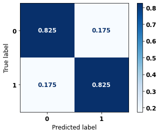
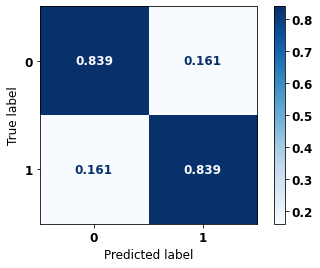
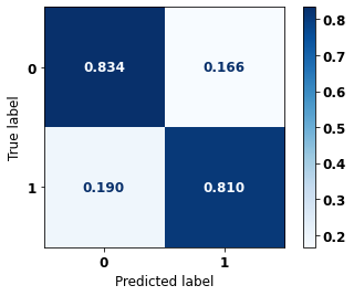
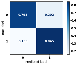
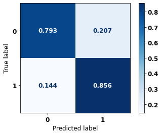
display_confusion_matrix(rf_sp, X_test_SP, y_test_SP)

              precision    recall  f1-score   support

           0      0.906     0.828     0.865     84231
           1      0.708     0.829     0.764     42279

    accuracy                          0.828    126510
   macro avg      0.807     0.829     0.814    126510
weighted avg      0.840     0.828     0.831    126510
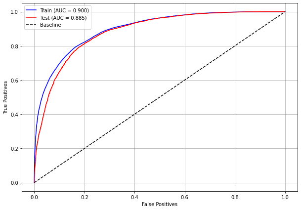
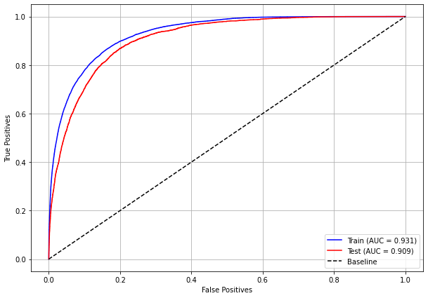
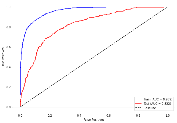
The confusion matrix obtained for the Random Forest, with SP data, shows a good performance of the model, with 83% of accuracy.
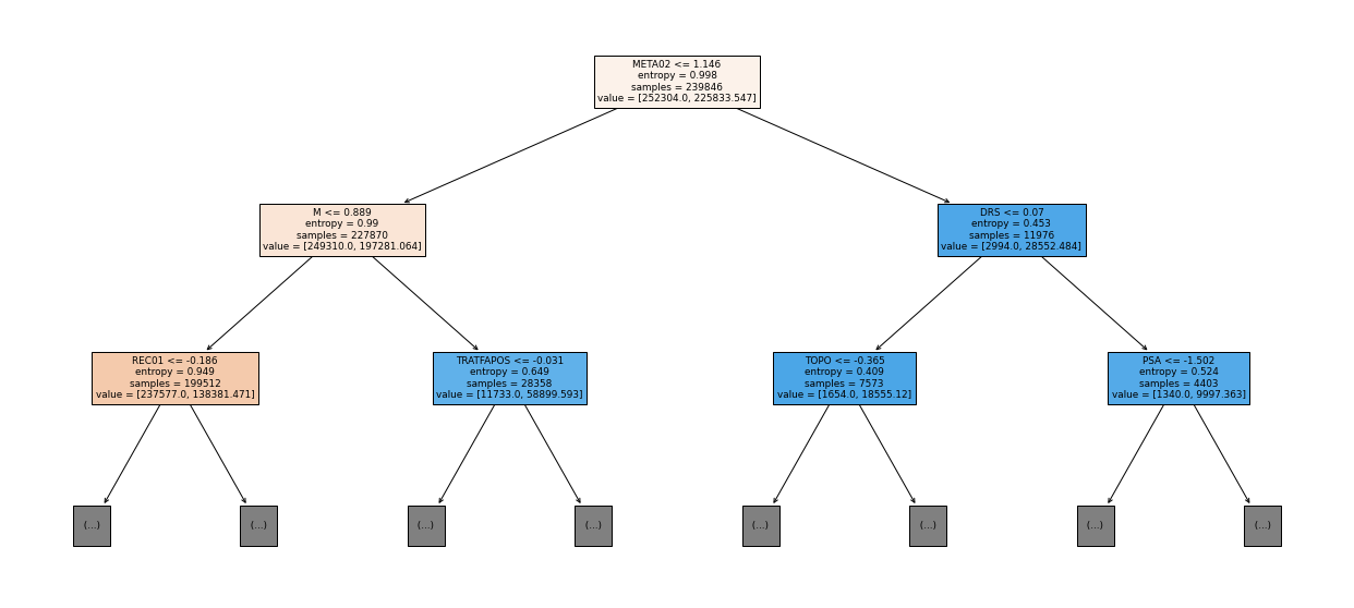
[ ]:
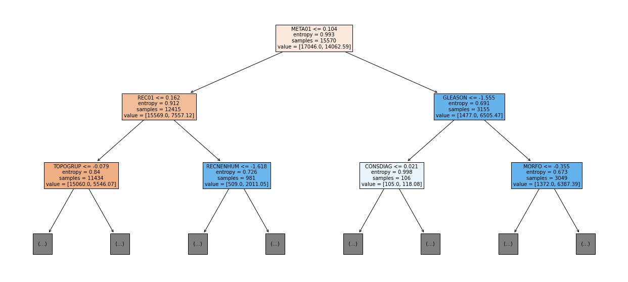
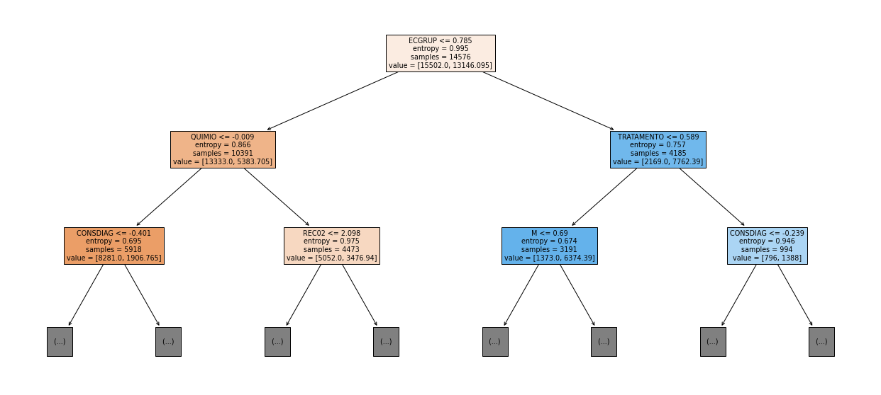
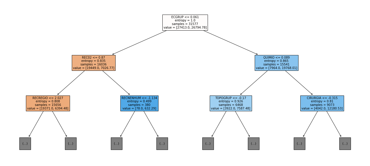
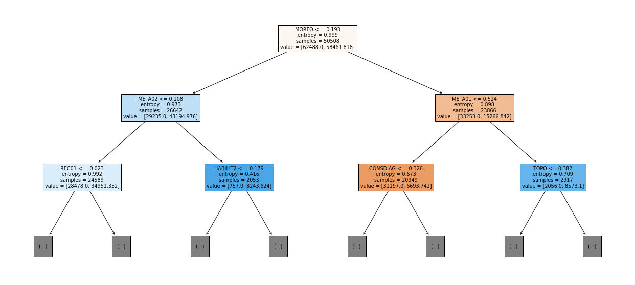
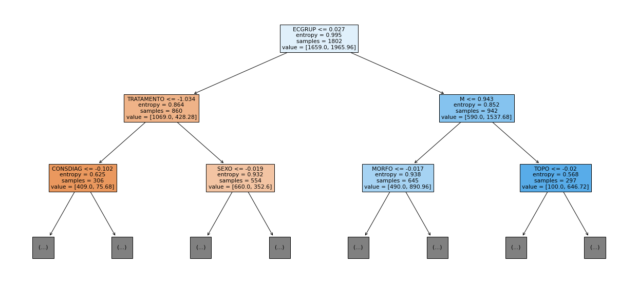
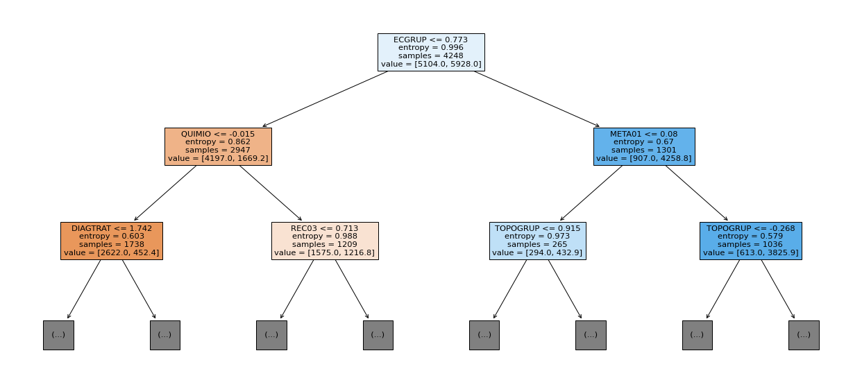
show_tree(rf_sp, feat_cols_SP, 2)
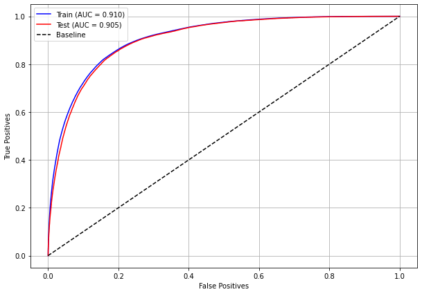
[ ]:
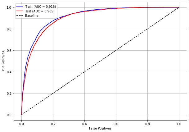
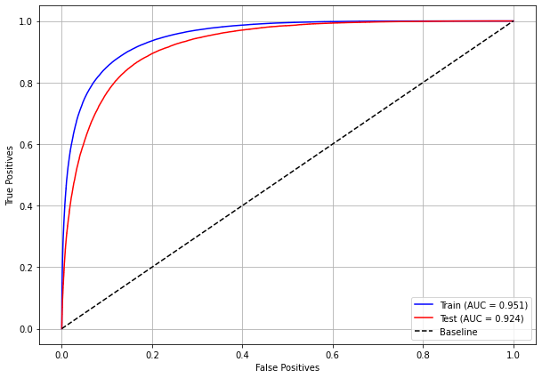
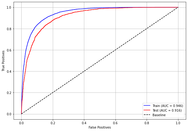
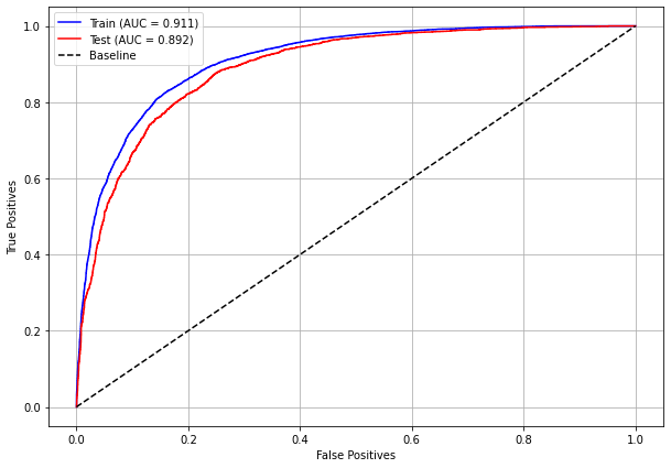
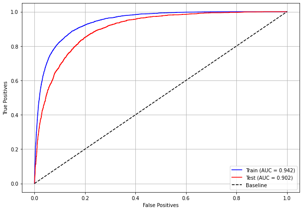
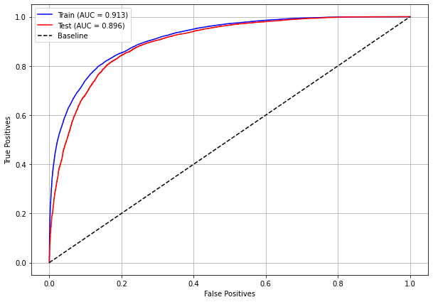
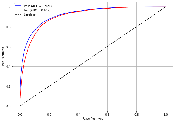
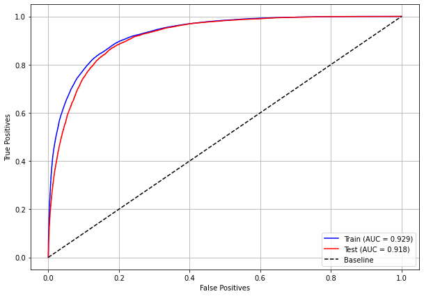
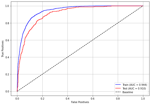
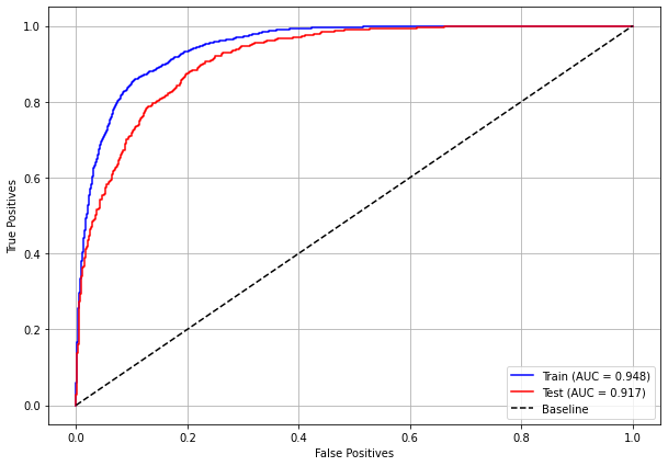
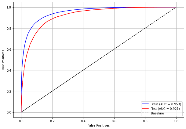
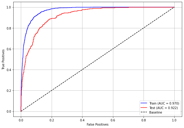
plot_roc_curve(rf_sp, X_train_SP, X_test_SP, y_train_SP, y_test_SP)
[ ]:
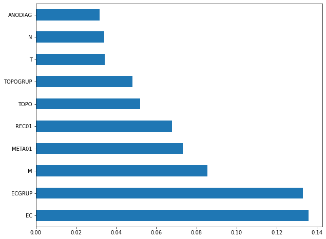
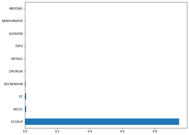
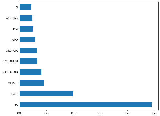
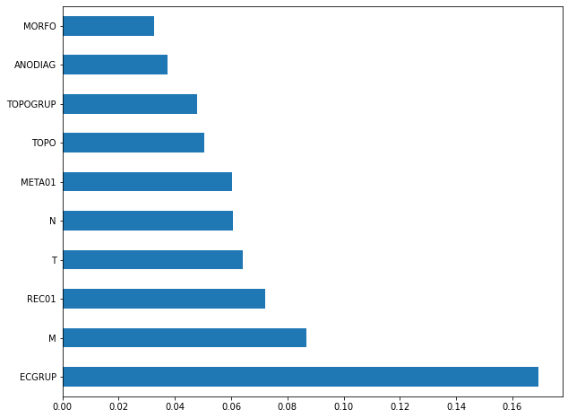
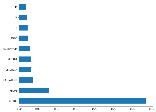
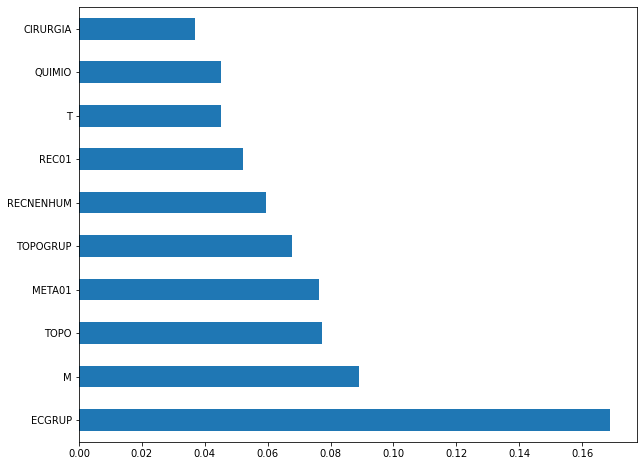
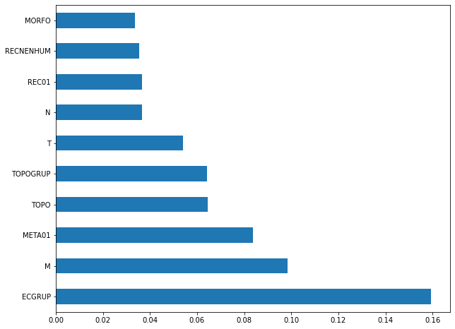
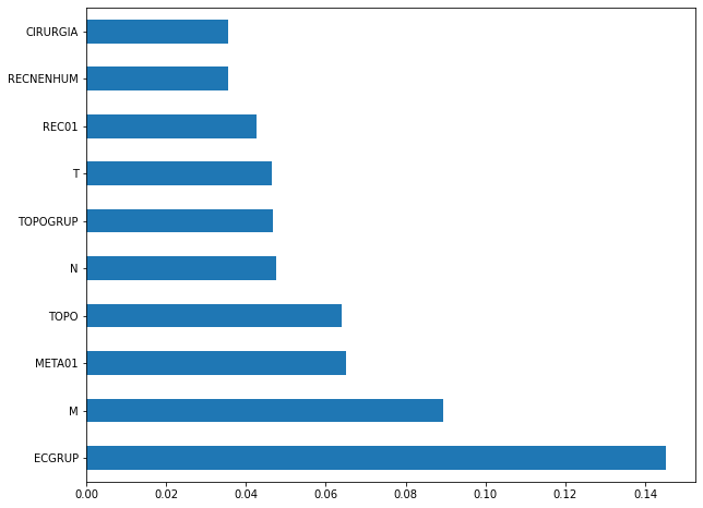
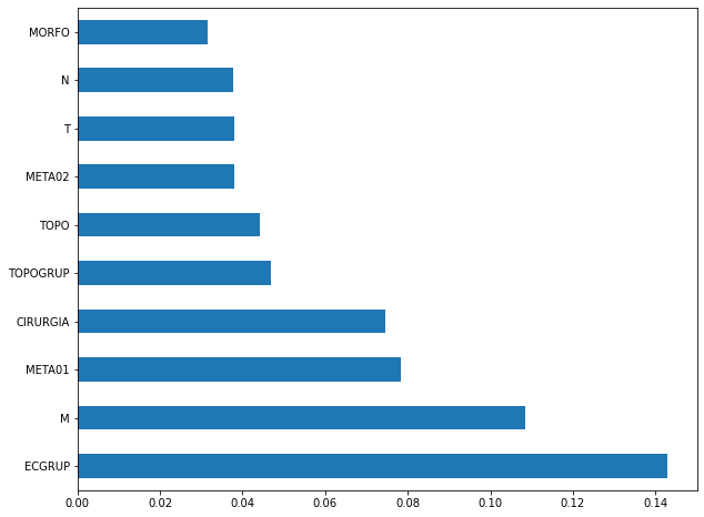
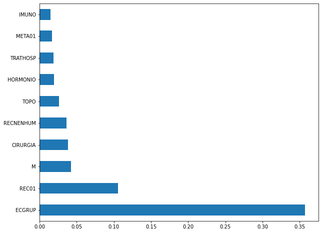
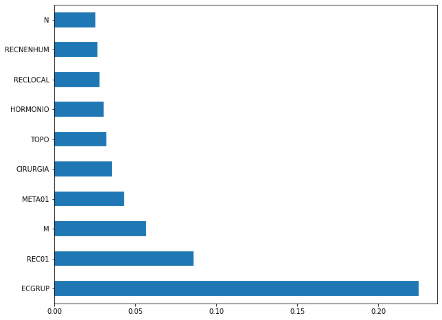
plot_feat_importances(rf_sp, feat_cols_SP)
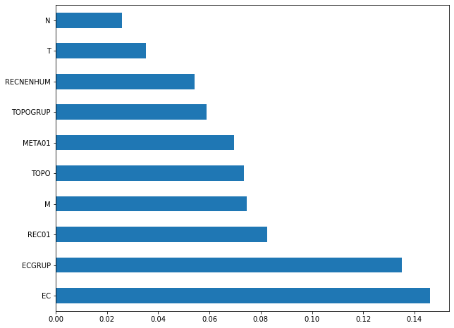
The four most important features in the model were
EC,ECGRUP,REC01andM.
[ ]:
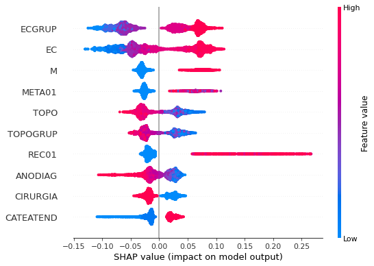
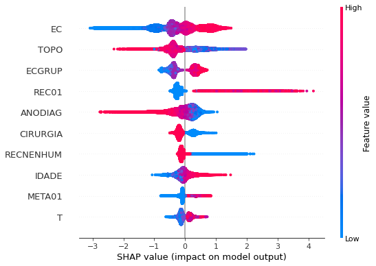
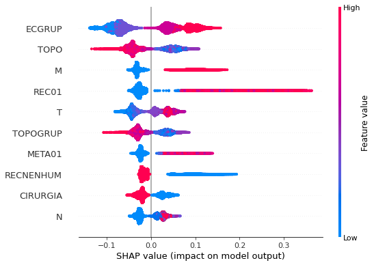
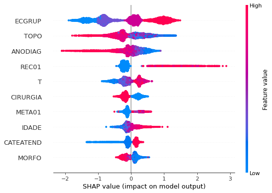
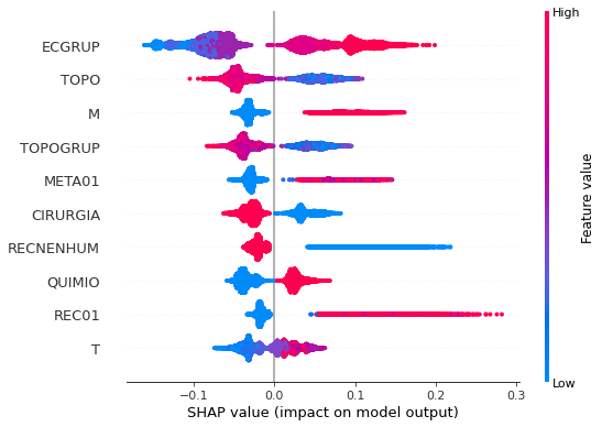
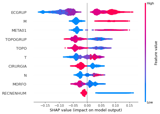
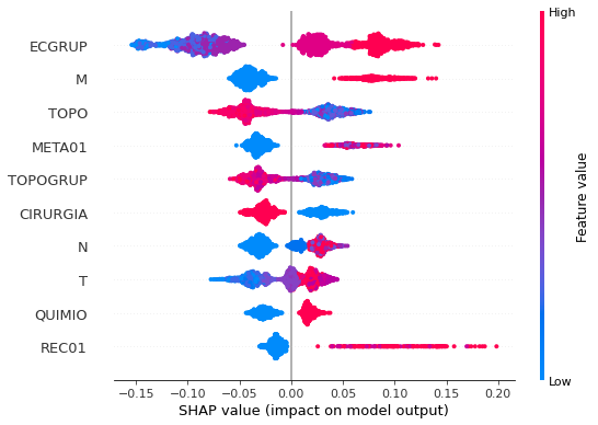
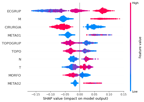
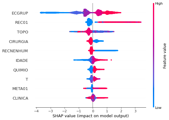
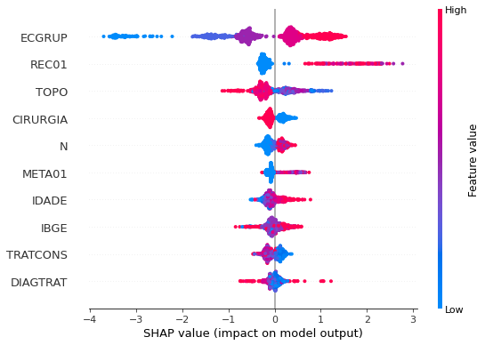
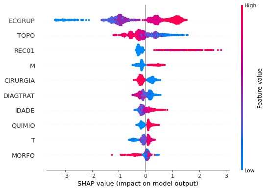
plot_shap_values(rf_sp, X_test_SP, feat_cols_SP)
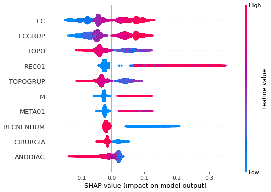
Note that larger values of the EC column, shown in pink, have more influence for the model’s prediction to be class 1, smaller values have greater weight for the prediction to be class 0. This behavior was expected, because the higher the clinical stage, worse is the stage of cancer.
The other columns shown follow the same logic.
[ ]:
# Other states
rf_fora = RandomForestClassifier(class_weight={0:1, 1:1.845},
                                 random_state=seed,
                                 criterion='entropy',
                                 max_depth=8)

rf_fora.fit(X_train_OS, y_train_OS)
RandomForestClassifier(class_weight={0: 1, 1: 1.845}, criterion='entropy',
                       max_depth=8, random_state=10)
[ ]:
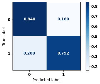
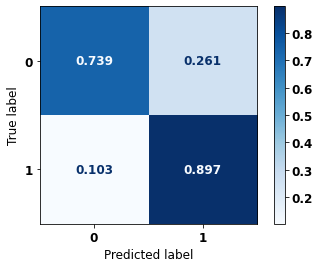
display_confusion_matrix(rf_fora, X_test_OS, y_test_OS)
              precision    recall  f1-score   support

           0      0.914     0.825     0.867      5701
           1      0.676     0.825     0.743      2522

    accuracy                          0.825      8223
   macro avg      0.795     0.825     0.805      8223
weighted avg      0.841     0.825     0.829      8223
The confusion matrix obtained for the Random Forest algorithm with the other states data shows a good performance of the model, because the model achieves a 82% of accuracy.
[ ]:
show_tree(rf_fora, feat_cols_OS, 2)
[ ]:
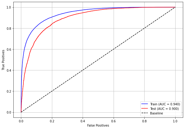
plot_roc_curve(rf_fora, X_train_OS, X_test_OS, y_train_OS, y_test_OS)
[ ]:
plot_feat_importances(rf_fora, feat_cols_OS)
The four most important features in the model were
EC,ECGRUP,MandMETA01.
[ ]:
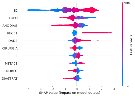
plot_shap_values(rf_fora, X_test_OS, feat_cols_OS)
Again larger values of the ECGRUP column, shown in pink, have more influence for the model’s prediction to be class 1, smaller values have greater weight for the prediction to be class 0. This behavior was expected, because the higher the clinical stage, worse is the stage of cancer.
The other columns shown follow the same logic.
Randomized Grid Search
[ ]:
# RandomizedSearchCV
hyperRF = {'n_estimators': [100, 150, 200, 250],
           'max_depth': [5, 8, 10, 12, 15],
           'min_samples_split': [2, 5, 10, 15],
           'min_samples_leaf': [1, 2, 5, 10]}

rf = RandomForestClassifier(random_state=seed, criterion='entropy')

randRS = RandomizedSearchCV(rf, hyperRF, n_iter=20, cv=5, n_jobs=-1,
                            random_state=seed)
[ ]:
# SP
bestSP = randRS.fit(X_train_SP, y_train_SP)
[ ]:
bestSP.best_params_
{'n_estimators': 200,
 'min_samples_split': 10,
 'min_samples_leaf': 2,
 'max_depth': 15}
[ ]:
# SP
rf_sp_opt = bestSP.best_estimator_
rf_sp_opt.set_params(class_weight={0:1, 1:1.85})

rf_sp_opt.fit(X_train_SP, y_train_SP)
RandomForestClassifier(class_weight={0: 1, 1: 1.85}, criterion='entropy',
                       max_depth=15, min_samples_leaf=2, min_samples_split=10,
                       n_estimators=200, random_state=10)
[ ]:
display_confusion_matrix(rf_sp_opt, X_test_SP, y_test_SP)
              precision    recall  f1-score   support

           0      0.912     0.839     0.874     84231
           1      0.723     0.839     0.777     42279

    accuracy                          0.839    126510
   macro avg      0.818     0.839     0.825    126510
weighted avg      0.849     0.839     0.842    126510
[ ]:
# Other States
bestOS = randRS.fit(X_train_OS, y_train_OS)
[ ]:
bestOS.best_params_
{'n_estimators': 200,
 'min_samples_split': 10,
 'min_samples_leaf': 2,
 'max_depth': 15}
[ ]:
# Other states
rf_fora_opt = bestOS.best_estimator_
rf_fora_opt.set_params(class_weight={0:1, 1:2.58})

rf_fora_opt.fit(X_train_OS, y_train_OS)
RandomForestClassifier(class_weight={0: 1, 1: 2.58}, criterion='entropy',
                       max_depth=15, min_samples_leaf=2, min_samples_split=10,
                       n_estimators=200, random_state=10)
[ ]:
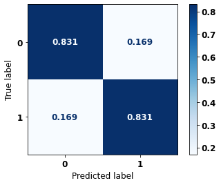
display_confusion_matrix(rf_fora_opt, X_test_OS, y_test_OS)

              precision    recall  f1-score   support

           0      0.919     0.835     0.875      5701
           1      0.691     0.834     0.756      2522

    accuracy                          0.835      8223
   macro avg      0.805     0.835     0.815      8223
weighted avg      0.849     0.835     0.839      8223
XGBoost
The training of the XGBoost model follows the same pattern with random_state. A higher weight was also used for the class with fewer examples, using the hyperparameter scale_pos_weight.
The hyperparameter max_depth was chosen as 10 because the default value for this hyperparameter is 3, a low value for the amount of data we have.
[ ]:
# SP
xgboost_sp = XGBClassifier(max_depth=10,
                           scale_pos_weight=1.89,
                           random_state=seed)

xgboost_sp.fit(X_train_SP, y_train_SP)
XGBClassifier(max_depth=10, random_state=10, scale_pos_weight=1.89)
[ ]:
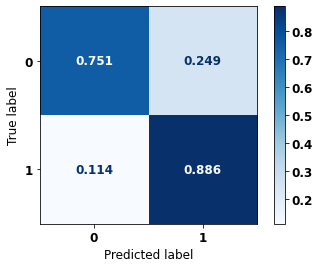
display_confusion_matrix(xgboost_sp, X_test_SP, y_test_SP)

              precision    recall  f1-score   support

           0      0.918     0.849     0.882     84231
           1      0.738     0.849     0.790     42279

    accuracy                          0.849    126510
   macro avg      0.828     0.849     0.836    126510
weighted avg      0.858     0.849     0.851    126510
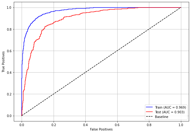
The confusion matrix obtained for the XGBoost, with SP data, also shows a good performance of the model, with 85% of accuracy.
[ ]:
plot_roc_curve(xgboost_sp, X_train_SP, X_test_SP, y_train_SP, y_test_SP)
[ ]:
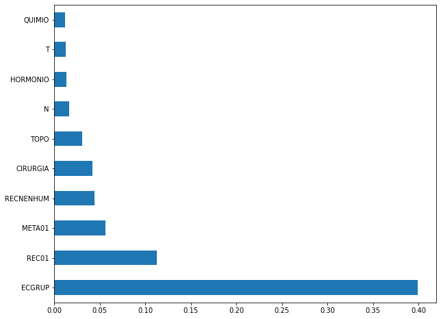
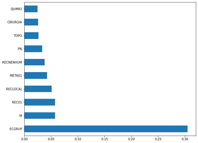
plot_feat_importances(xgboost_sp, feat_cols_SP)
The four most important features in the model were
ECGRUP, with a lot advantage over the others,REC01,ECandRECNENHUM.
[ ]:
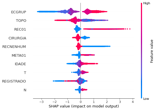
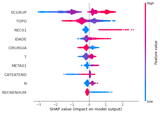
plot_shap_values(xgboost_sp, X_test_SP, feat_cols_SP)
Note that larger values of the EC column, shown in pink, have more influence for the model’s prediction to be class 1, smaller values have greater weight for the prediction to be class 0. This behavior was expected, because the higher the clinical stage, worse is the stage of cancer.
The other columns shown follow the same logic.
[ ]:
# Other states
xgboost_fora = XGBClassifier(max_depth=6,
                             scale_pos_weight=2,
                             random_state=seed)

xgboost_fora.fit(X_train_OS, y_train_OS)
XGBClassifier(max_depth=6, random_state=10, scale_pos_weight=2)
[ ]:
display_confusion_matrix(xgboost_fora, X_test_OS, y_test_OS)

              precision    recall  f1-score   support

           0      0.921     0.838     0.878      5701
           1      0.696     0.838     0.761      2522

    accuracy                          0.838      8223
   macro avg      0.809     0.838     0.819      8223
weighted avg      0.852     0.838     0.842      8223
The confusion matrix obtained for the XGBoost algorithm with SP data shows a good performance of the model, because the model achieves a 84% of accuracy.
[ ]:
plot_roc_curve(xgboost_fora, X_train_OS, X_test_OS, y_train_OS, y_test_OS)
[ ]:
plot_feat_importances(xgboost_fora, feat_cols_OS)
The four most important features in the model were
EC, with a good advantage,REC01,META01andCATEATEND.
[ ]:
plot_shap_values(xgboost_fora, X_test_OS, feat_cols_OS)
Note that larger values of the EC column, shown in pink, have more influence for the model’s prediction to be class 1, smaller values have greater weight for the prediction to be class 0. This behavior was expected, because the higher the clinical stage, worse is the stage of cancer.
The other columns shown follow the same logic.
Randomized Grid Search
[ ]:
# RandomizedSearchCV
hyperXGB = {'learning_rate': [0.05, 0.10, 0.15, 0.20],
            'max_depth': [5, 8, 10, 12, 15],
            'min_child_weight': [1, 3, 5, 7],
            'gamma': [0.0, 0.1, 0.2 , 0.3],
            'colsample_bytree': [0.3, 0.4, 0.5, 0.7],
            'n_estimators': [100, 150, 200, 250]}

xgboost = XGBClassifier(random_state=seed)
xgbRS = RandomizedSearchCV(xgboost, hyperXGB, n_iter=20, cv=5, n_jobs=-1,
                           random_state=seed)
[ ]:
# SP
bestSP = xgbRS.fit(X_train_SP, y_train_SP)
[ ]:
bestSP.best_params_
{'n_estimators': 200,
 'min_child_weight': 5,
 'max_depth': 10,
 'learning_rate': 0.1,
 'gamma': 0.2,
 'colsample_bytree': 0.4}
[ ]:
# SP
xgb_sp_opt = bestSP.best_estimator_
xgb_sp_opt.set_params(scale_pos_weight=1.88)

xgb_sp_opt.fit(X_train_SP, y_train_SP)
XGBClassifier(colsample_bytree=0.4, gamma=0.2, max_depth=10, min_child_weight=5,
              n_estimators=200, random_state=10, scale_pos_weight=1.88)
[ ]:
display_confusion_matrix(xgb_sp_opt, X_test_SP, y_test_SP)

              precision    recall  f1-score   support

           0      0.919     0.852     0.884     84231
           1      0.742     0.851     0.793     42279

    accuracy                          0.851    126510
   macro avg      0.831     0.851     0.839    126510
weighted avg      0.860     0.851     0.854    126510
[ ]:
# Other States
bestOS = xgbRS.fit(X_train_OS, y_train_OS)
[ ]:
bestOS.best_params_
{'n_estimators': 150,
 'min_child_weight': 5,
 'max_depth': 5,
 'learning_rate': 0.1,
 'gamma': 0.2,
 'colsample_bytree': 0.4}
[ ]:
# Other states
xgb_fora_opt = bestOS.best_estimator_
xgb_fora_opt.set_params(scale_pos_weight=1.99)

xgb_fora_opt.fit(X_train_OS, y_train_OS)
XGBClassifier(colsample_bytree=0.4, gamma=0.2, max_depth=5, min_child_weight=5,
              n_estimators=150, random_state=10, scale_pos_weight=1.99)
[ ]:
display_confusion_matrix(xgb_fora_opt, X_test_OS, y_test_OS)
              precision    recall  f1-score   support

           0      0.923     0.841     0.880      5701
           1      0.700     0.843     0.765      2522

    accuracy                          0.841      8223
   macro avg      0.812     0.842     0.823      8223
weighted avg      0.855     0.841     0.845      8223
Second approach
Approach using only morphologies with final digit equal to 3 and without EC column as a feature.
Preprocessing
Now we are going to divide the data into training and testing, and then do the preprocessing in both datasets to perform the training of the models and their evaluation.
First, it is necessary to define the columns that will be used as features and the label. We will not use some columns of the data: UFRESID, because we already have the division between SP and other states in the two datasets.
It was chosen to keep the column IDADE, so we will not use the FAIXAETAR, as well as the column ECGRUP and not the column EC. Finally, the other columns contained in the list list_drop are possible labels, so they will not be used as features for machine learning models.
[ ]:
list_drop = ['UFRESID', 'FAIXAETAR', 'ULTICONS', 'ULTIDIAG', 'ULTITRAT',
             'vivo_ano1', 'vivo_ano3', 'vivo_ano5', 'ULTINFO', 'EC', 'obito_geral']

lb = 'obito_cancer'
A function was created to perform the preprocessing, preprocessing, that uses the other functions created, get_train_test (divides the dataset into train and test sets), train_preprocessing (do the preprocessing of the train set) and test_preprocessing (do the preprocessing of the test set).
To see the complete function go to the functions section.
SP
[ ]:
X_train_SP, X_test_SP, y_train_SP, y_test_SP, feat_cols_SP = preprocessing(df_SP, list_drop, lb,
                                                                           morpho3=True,
                                                                           random_state=seed,
                                                                           balance_data=False,
                                                                           encoder_type='LabelEncoder',
                                                                           norm_name='StandardScaler')
X_train = (351486, 65), X_test = (117163, 65)
y_train = (351486,), y_test = (117163,)
Other states
[ ]:
X_train_OS, X_test_OS, y_train_OS, y_test_OS, feat_cols_OS = preprocessing(df_fora, list_drop, lb,
                                                                           morpho3=True,
                                                                           random_state=seed,
                                                                           balance_data=False,
                                                                           encoder_type='LabelEncoder',
                                                                           norm_name='StandardScaler')
X_train = (23079, 65), X_test = (7693, 65)
y_train = (23079,), y_test = (7693,)
Training machine learning models
After dividing the data into training and testing, using the encoder and normalizing, the data is ready to be used by the machine learning models.
Random Forest
The first model that will be tested is the Random Forest, for this test the parameter random_state will be used, to obtain the same training values of the model every time it is runned.
The hyperparameter class_weight was also used because the model has difficulty learning the class with fewer examples, so using this parameter this class will have a higher weight in the training of the model.
[ ]:
# SP
rf_sp = RandomForestClassifier(random_state=seed,
                               class_weight={0:1, 1:1.685},
                               criterion='entropy',
                               max_depth=10)

rf_sp.fit(X_train_SP, y_train_SP)
RandomForestClassifier(class_weight={0: 1, 1: 1.685}, criterion='entropy',
                       max_depth=10, random_state=10)
[ ]:
display_confusion_matrix(rf_sp, X_test_SP, y_test_SP)

              precision    recall  f1-score   support

           0      0.890     0.818     0.853     75153
           1      0.716     0.819     0.764     42010

    accuracy                          0.818    117163
   macro avg      0.803     0.819     0.808    117163
weighted avg      0.828     0.818     0.821    117163
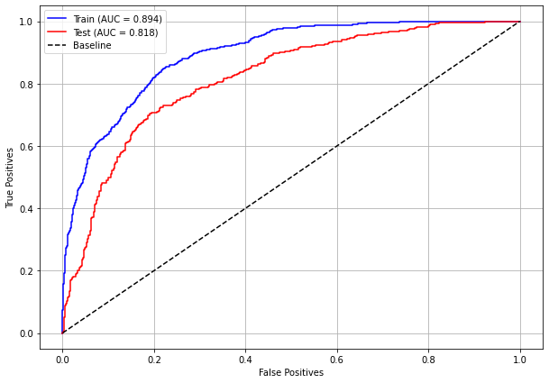
The confusion matrix obtained for the Random Forest, with SP data, also shows a good performance of the model, with 82% of accuracy.
[ ]:
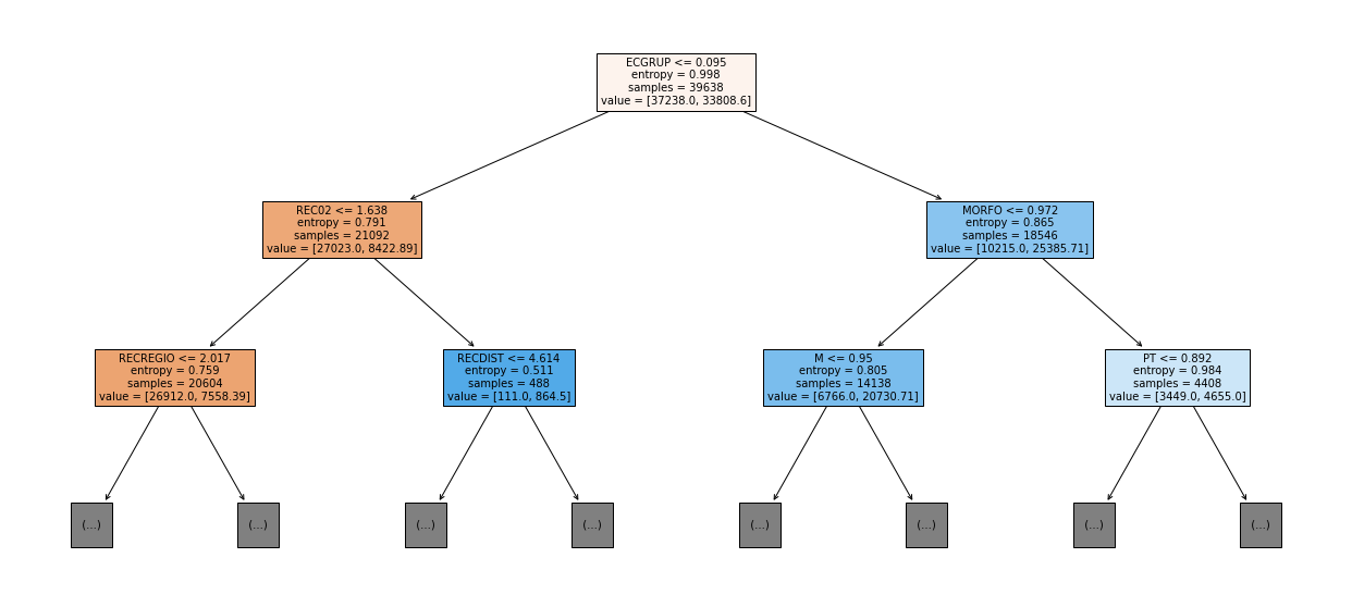
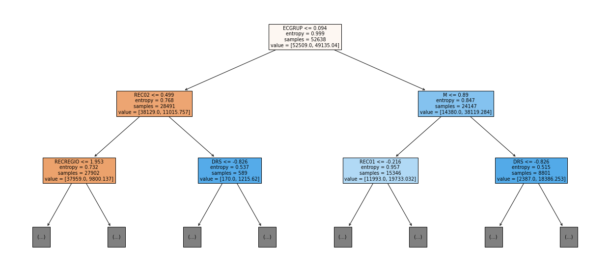
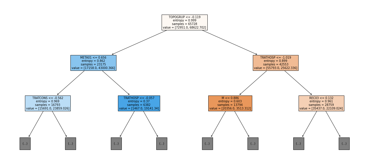
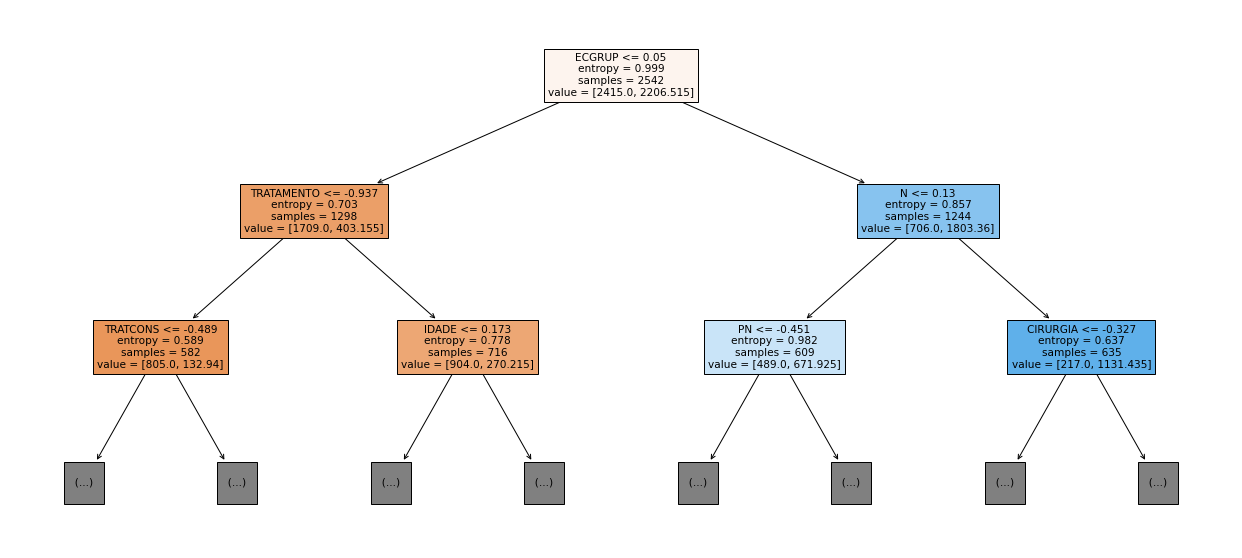
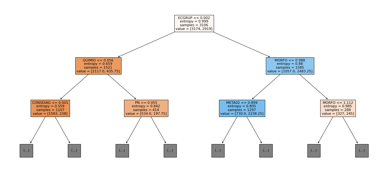
show_tree(rf_sp, feat_cols_SP, 2)
[ ]:
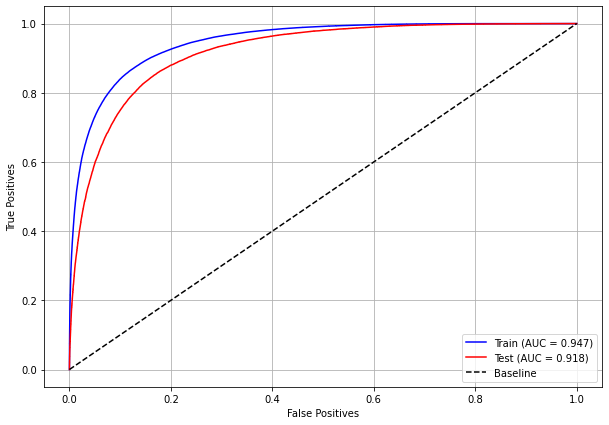
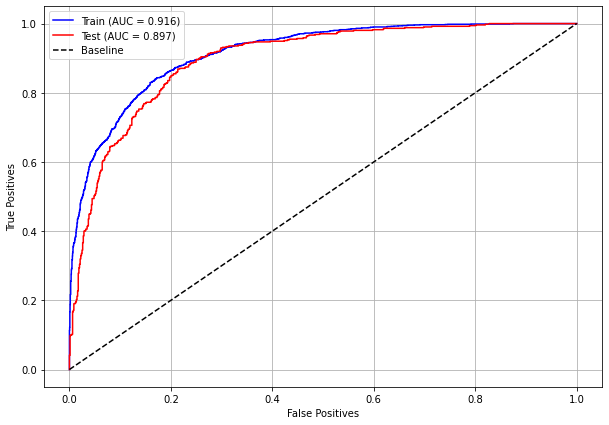
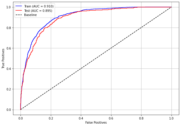
plot_roc_curve(rf_sp, X_train_SP, X_test_SP, y_train_SP, y_test_SP)
[ ]:
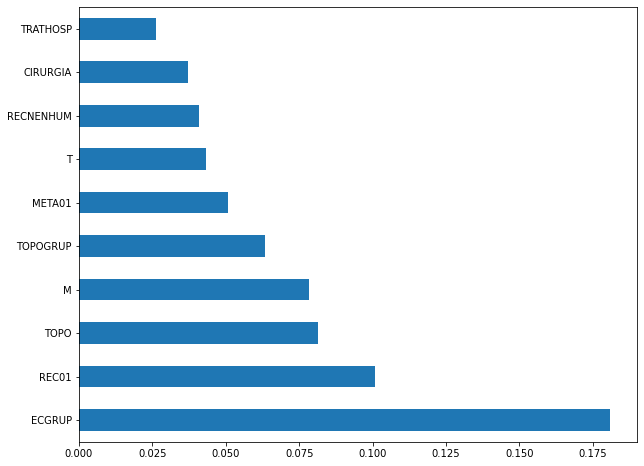
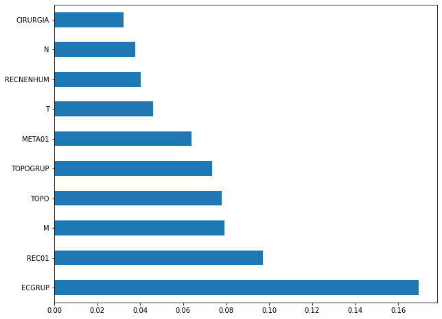
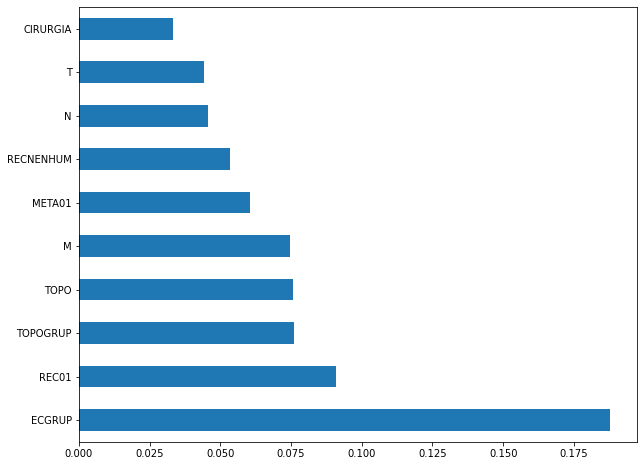
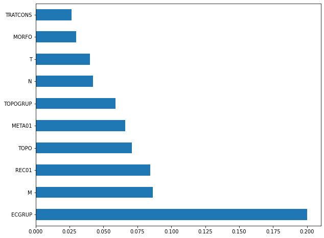
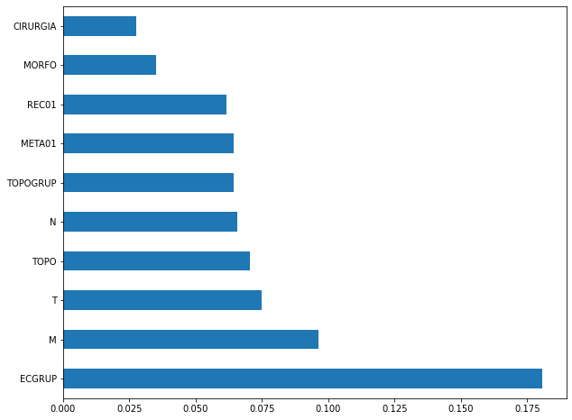
plot_feat_importances(rf_sp, feat_cols_SP)
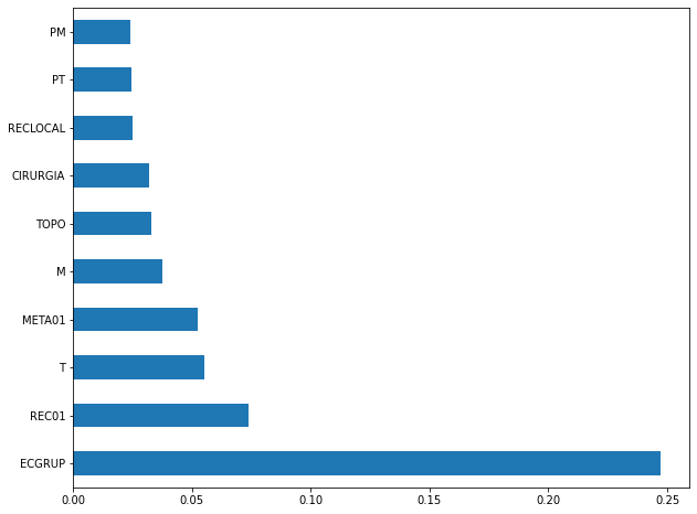
The four most important features in the model were
ECGRUP,REC01,MandT.
[ ]:
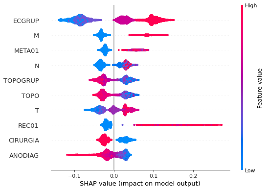
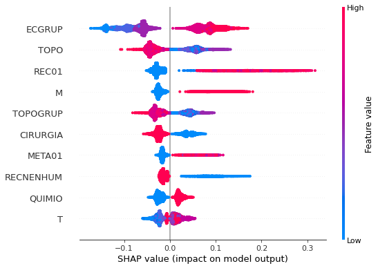
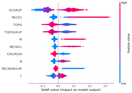
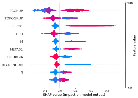
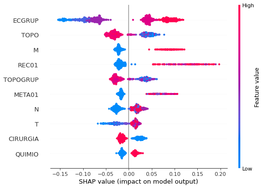
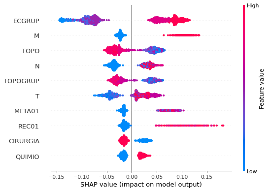
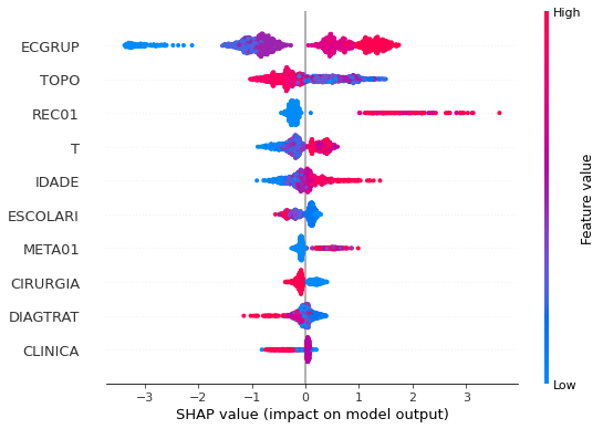
plot_shap_values(rf_sp, X_test_SP, feat_cols_SP)
Note that larger values of the ECGRUP column, shown in pink, have more influence for the model’s prediction to be class 1, smaller values have greater weight for the prediction to be class 0. This behavior was expected, because the higher the clinical stage, worse is the stage of cancer.
The other columns shown follow the same logic.
[ ]:
# Other states
rf_fora = RandomForestClassifier(random_state=seed,
                                 class_weight={0:1, 1:1.735},
                                 criterion='entropy',
                                 max_depth=8)

rf_fora.fit(X_train_OS, y_train_OS)
RandomForestClassifier(class_weight={0: 1, 1: 1.735}, criterion='entropy',
                       max_depth=8, random_state=10)
[ ]:
display_confusion_matrix(rf_fora, X_test_OS, y_test_OS)

              precision    recall  f1-score   support

           0      0.898     0.810     0.852      5176
           1      0.675     0.810     0.736      2517

    accuracy                          0.810      7693
   macro avg      0.786     0.810     0.794      7693
weighted avg      0.825     0.810     0.814      7693
The confusion matrix obtained for the Random Forest algorithm with other states data shows a good performance of the model, because the model achieves a 81% of accuracy.
[ ]:
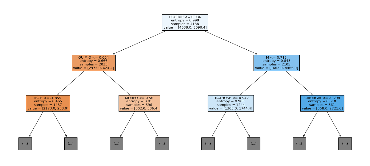
show_tree(rf_fora, feat_cols_OS, 2)
[ ]:
plot_roc_curve(rf_fora, X_train_OS, X_test_OS, y_train_OS, y_test_OS)
[ ]:
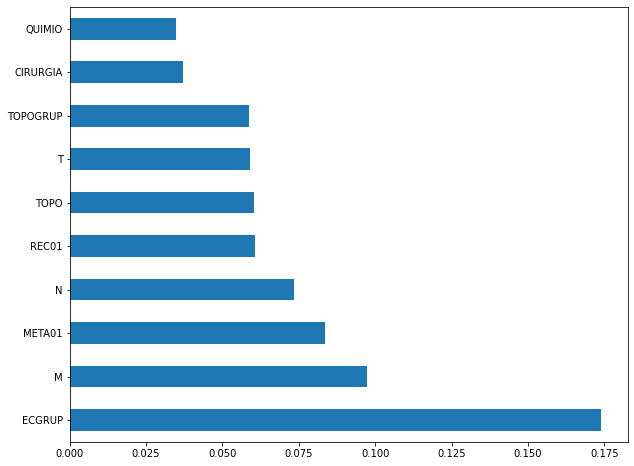
plot_feat_importances(rf_fora, feat_cols_OS)
The four most important features in the model were
ECGRUP,M,REC01andT.
[ ]:
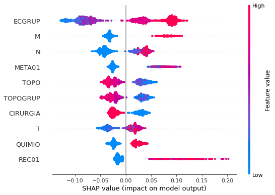
plot_shap_values(rf_fora, X_test_OS, feat_cols_OS)
Note that larger values of the ECGRUP column, shown in pink, have more influence for the model’s prediction to be class 1, smaller values have greater weight for the prediction to be class 0. This behavior was expected, because the higher the clinical stage, worse is the stage of cancer.
The other columns shown follow the same logic.
XGBoost
The training of the XGBoost model follows the same pattern with random_state. A higher weight was also used for the class with fewer examples, using the hyperparameter scale_pos_weight.
The hyperparameter max_depth was chosen as 10 because the default value for this hyperparameter is 3, a low value for the amount of data we have.
[ ]:
# SP
xgboost_sp = XGBClassifier(max_depth=10,
                           scale_pos_weight=1.7,
                           random_state=seed)

xgboost_sp.fit(X_train_SP, y_train_SP)
XGBClassifier(max_depth=10, random_state=10, scale_pos_weight=1.7)
[ ]:
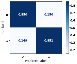
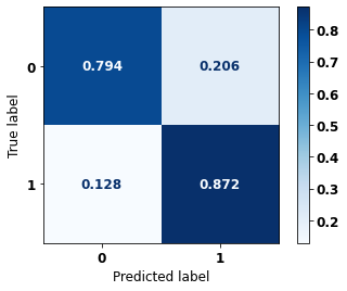
display_confusion_matrix(xgboost_sp, X_test_SP, y_test_SP)

              precision    recall  f1-score   support

           0      0.904     0.842     0.872     75153
           1      0.749     0.841     0.792     42010

    accuracy                          0.842    117163
   macro avg      0.826     0.841     0.832    117163
weighted avg      0.848     0.842     0.843    117163
The confusion matrix obtained for the XGBoost, with SP data, also shows a good performance of the model, with 84% of accuracy.
[ ]:
plot_roc_curve(xgboost_sp, X_train_SP, X_test_SP, y_train_SP, y_test_SP)
[ ]:
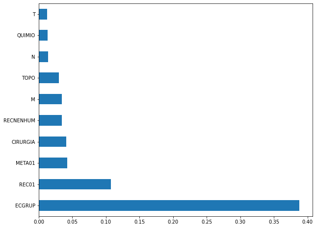
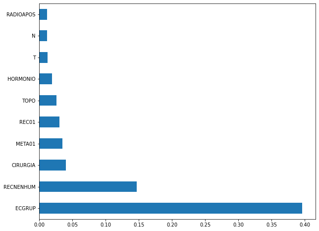
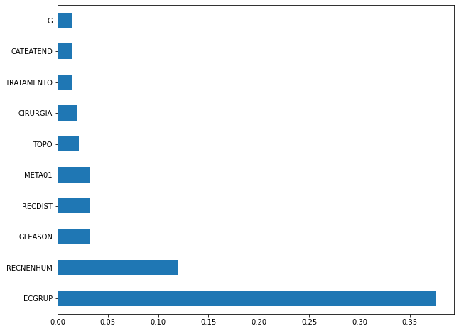
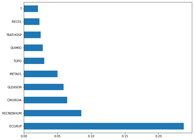
plot_feat_importances(xgboost_sp, feat_cols_SP)
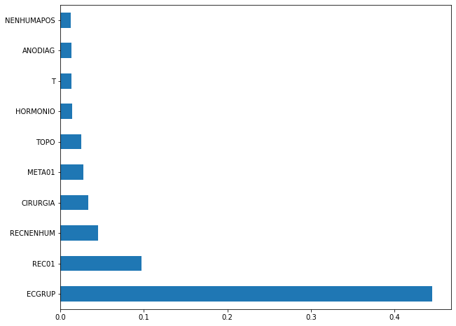
The four most important features in the model were
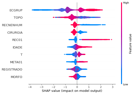
ECGRUP,REC01,RECNENHUMandCIRURGIA.
[ ]:
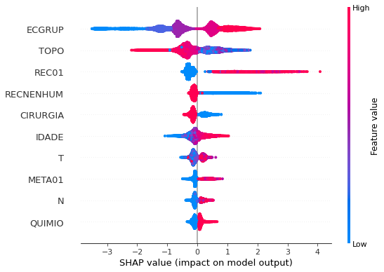
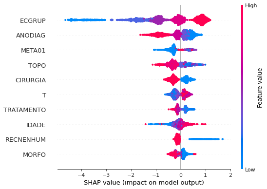
plot_shap_values(xgboost_sp, X_test_SP, feat_cols_SP)
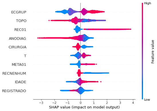
Note that larger values of the ECGRUP column, shown in pink, have more influence for the model’s prediction to be class 1, smaller values have greater weight for the prediction to be class 0. This behavior was expected, because the higher the clinical stage, worse is the stage of cancer.
The other columns shown follow the same logic.
[ ]:
# Other states
xgboost_fora = XGBClassifier(max_depth=6,
                             scale_pos_weight=1.87,
                             random_state=seed)

xgboost_fora.fit(X_train_OS, y_train_OS)
XGBClassifier(max_depth=6, random_state=10, scale_pos_weight=1.87)
[ ]:
display_confusion_matrix(xgboost_fora, X_test_OS, y_test_OS)

              precision    recall  f1-score   support

           0      0.905     0.823     0.862      5176
           1      0.693     0.822     0.752      2517

    accuracy                          0.823      7693
   macro avg      0.799     0.823     0.807      7693
weighted avg      0.836     0.823     0.826      7693
The confusion matrix obtained for the XGBoost algorithm with SP data shows a good performance of the model, because the model achieves a 82% of accuracy.
[ ]:
plot_roc_curve(xgboost_fora, X_train_OS, X_test_OS, y_train_OS, y_test_OS)
[ ]:
plot_feat_importances(xgboost_fora, feat_cols_OS)
The four most important features in the model were
ECGRUP,REC01,CATEATENDandCIRURGIA.
[ ]:
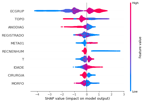
plot_shap_values(xgboost_fora, X_test_OS, feat_cols_OS)
Note that larger values of the ECGRUP column, shown in pink, have more influence for the model’s prediction to be class 1, smaller values have greater weight for the prediction to be class 0. This behavior was expected, because the higher the clinical stage, worse is the stage of cancer.
The other columns shown follow the same logic.
Third approach
Approach with grouped years and without the column EC.
Preprocessing
Now we are going to divide the data into training and testing, and then do the preprocessing in both datasets to perform the training of the models and their evaluation. We will use the years grouped too, resulting in 5 datasets for SP and more 5 for other states.
First, it is necessary to define the columns that will be used as features and the label. We will not use some columns of the data: UFRESID, because we already have the division between SP and other states in the two datasets.
It was chosen to keep the column IDADE, so we will not use the FAIXAETAR, as well as the column ECGRUP and not the column EC. Finally, the other columns contained in the list list_drop are possible labels, so they will not be used as features for machine learning models.
[ ]:
list_drop = ['UFRESID', 'FAIXAETAR', 'ULTICONS', 'ULTIDIAG', 'ULTITRAT',
             'vivo_ano1', 'vivo_ano3', 'vivo_ano5', 'ULTINFO', 'EC', 'obito_geral']

lb = 'obito_cancer'
A function was created to perform the preprocessing, preprocessing, that uses the other functions created, get_train_test (divides the dataset into train and test sets), train_preprocessing (do the preprocessing of the train set) and test_preprocessing (do the preprocessing of the test set).
The process will be done 5 times for SP and other states, using the datasets with grouped years.
To see the complete function go to the functions section.
SP
[ ]:
X_trainSP_00_03, X_testSP_00_03, y_trainSP_00_03, y_testSP_00_03, feat_SP_00_03 = preprocessing(df_SP, list_drop, lb,
                                                                                                group_years=True,
                                                                                                first_year=2000,
                                                                                                last_year=2003,
                                                                                                random_state=seed,
                                                                                                balance_data=False,
                                                                                                encoder_type='LabelEncoder',
                                                                                                norm_name='StandardScaler')
X_train = (49873, 65), X_test = (16625, 65)
y_train = (49873,), y_test = (16625,)
[ ]:
X_trainSP_04_07, X_testSP_04_07, y_trainSP_04_07, y_testSP_04_07, feat_SP_04_07 = preprocessing(df_SP, list_drop, lb,
                                                                                                group_years=True,
                                                                                                first_year=2004,
                                                                                                last_year=2007,
                                                                                                random_state=seed,
                                                                                                balance_data=False,
                                                                                                encoder_type='LabelEncoder',
                                                                                                norm_name='StandardScaler')
X_train = (62658, 65), X_test = (20887, 65)
y_train = (62658,), y_test = (20887,)
[ ]:
X_trainSP_08_11, X_testSP_08_11, y_trainSP_08_11, y_testSP_08_11, feat_SP_08_11 = preprocessing(df_SP, list_drop, lb,
                                                                                                group_years=True,
                                                                                                first_year=2008,
                                                                                                last_year=2011,
                                                                                                random_state=seed,
                                                                                                balance_data=False,
                                                                                                encoder_type='LabelEncoder',
                                                                                                norm_name='StandardScaler')
X_train = (83228, 65), X_test = (27743, 65)
y_train = (83228,), y_test = (27743,)
[ ]:
X_trainSP_12_15, X_testSP_12_15, y_trainSP_12_15, y_testSP_12_15, feat_SP_12_15 = preprocessing(df_SP, list_drop, lb,
                                                                                                group_years=True,
                                                                                                first_year=2012,
                                                                                                last_year=2015,
                                                                                                random_state=seed,
                                                                                                balance_data=False,
                                                                                                encoder_type='LabelEncoder',
                                                                                                norm_name='StandardScaler')
X_train = (103890, 65), X_test = (34630, 65)
y_train = (103890,), y_test = (34630,)
[ ]:
X_trainSP_16_21, X_testSP_16_21, y_trainSP_16_21, y_testSP_16_21, feat_SP_16_21 = preprocessing(df_SP, list_drop, lb,
                                                                                                group_years=True,
                                                                                                first_year=2016,
                                                                                                last_year=2021,
                                                                                                random_state=seed,
                                                                                                balance_data=False,
                                                                                                encoder_type='LabelEncoder',
                                                                                                norm_name='StandardScaler')
X_train = (79877, 65), X_test = (26626, 65)
y_train = (79877,), y_test = (26626,)
Other states
[ ]:
X_trainOS_00_03, X_testOS_00_03, y_trainOS_00_03, y_testOS_00_03, feat_OS_00_03 = preprocessing(df_fora, list_drop, lb,
                                                                                                group_years=True,
                                                                                                first_year=2000,
                                                                                                last_year=2003,
                                                                                                random_state=seed,
                                                                                                balance_data=False,
                                                                                                encoder_type='LabelEncoder',
                                                                                                norm_name='StandardScaler')
X_train = (2802, 65), X_test = (935, 65)
y_train = (2802,), y_test = (935,)
[ ]:
X_trainOS_04_07, X_testOS_04_07, y_trainOS_04_07, y_testOS_04_07, feat_OS_04_07 = preprocessing(df_fora, list_drop, lb,
                                                                                                group_years=True,
                                                                                                first_year=2004,
                                                                                                last_year=2007,
                                                                                                random_state=seed,
                                                                                                balance_data=False,
                                                                                                encoder_type='LabelEncoder',
                                                                                                norm_name='StandardScaler')
X_train = (3942, 65), X_test = (1315, 65)
y_train = (3942,), y_test = (1315,)
[ ]:
X_trainOS_08_11, X_testOS_08_11, y_trainOS_08_11, y_testOS_08_11, feat_OS_08_11 = preprocessing(df_fora, list_drop, lb,
                                                                                                group_years=True,
                                                                                                first_year=2008,
                                                                                                last_year=2011,
                                                                                                random_state=seed,
                                                                                                balance_data=False,
                                                                                                encoder_type='LabelEncoder',
                                                                                                norm_name='StandardScaler')
X_train = (4842, 65), X_test = (1614, 65)
y_train = (4842,), y_test = (1614,)
[ ]:
X_trainOS_12_15, X_testOS_12_15, y_trainOS_12_15, y_testOS_12_15, feat_OS_12_15 = preprocessing(df_fora, list_drop, lb,
                                                                                                group_years=True,
                                                                                                first_year=2012,
                                                                                                last_year=2015,
                                                                                                random_state=seed,
                                                                                                balance_data=False,
                                                                                                encoder_type='LabelEncoder',
                                                                                                norm_name='StandardScaler')
X_train = (6456, 65), X_test = (2153, 65)
y_train = (6456,), y_test = (2153,)
[ ]:
X_trainOS_16_20, X_testOS_16_20, y_trainOS_16_20, y_testOS_16_20, feat_OS_16_20 = preprocessing(df_fora, list_drop, lb,
                                                                                                group_years=True,
                                                                                                first_year=2016,
                                                                                                last_year=2020,
                                                                                                random_state=seed,
                                                                                                balance_data=False,
                                                                                                encoder_type='LabelEncoder',
                                                                                                norm_name='StandardScaler')
X_train = (6624, 65), X_test = (2208, 65)
y_train = (6624,), y_test = (2208,)
Training and evaluation of the models
After dividing the data into training and testing, using the encoder and normalizing, the data is ready to be used by the machine learning models.
Random Forest
The first model is the Random Forest, the random_state will be used as a parameter, to obtain the same training values of the model every time it is runned.
The hyperparameter class_weight was used because the models still have difficulty to learn the class with fewer examples.
SP
[ ]:
# SP - 2000 to 2003
rf_sp_00_03 = RandomForestClassifier(random_state=seed,
                                     class_weight={0:1, 1:1.193},
                                     criterion='entropy',
                                     max_depth=10)

rf_sp_00_03.fit(X_trainSP_00_03, y_trainSP_00_03)
RandomForestClassifier(class_weight={0: 1, 1: 1.193}, criterion='entropy',
                       max_depth=10, random_state=10)
[ ]:
display_confusion_matrix(rf_sp_00_03, X_testSP_00_03, y_testSP_00_03)

              precision    recall  f1-score   support

           0      0.837     0.807     0.821      9182
           1      0.772     0.806     0.788      7443

    accuracy                          0.806     16625
   macro avg      0.804     0.806     0.805     16625
weighted avg      0.808     0.806     0.807     16625
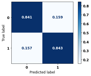
The confusion matrix obtained for the Random Forest, with SP data from 2000 to 2003, shows a good performance of the model, with 81% of accuracy.
[ ]:
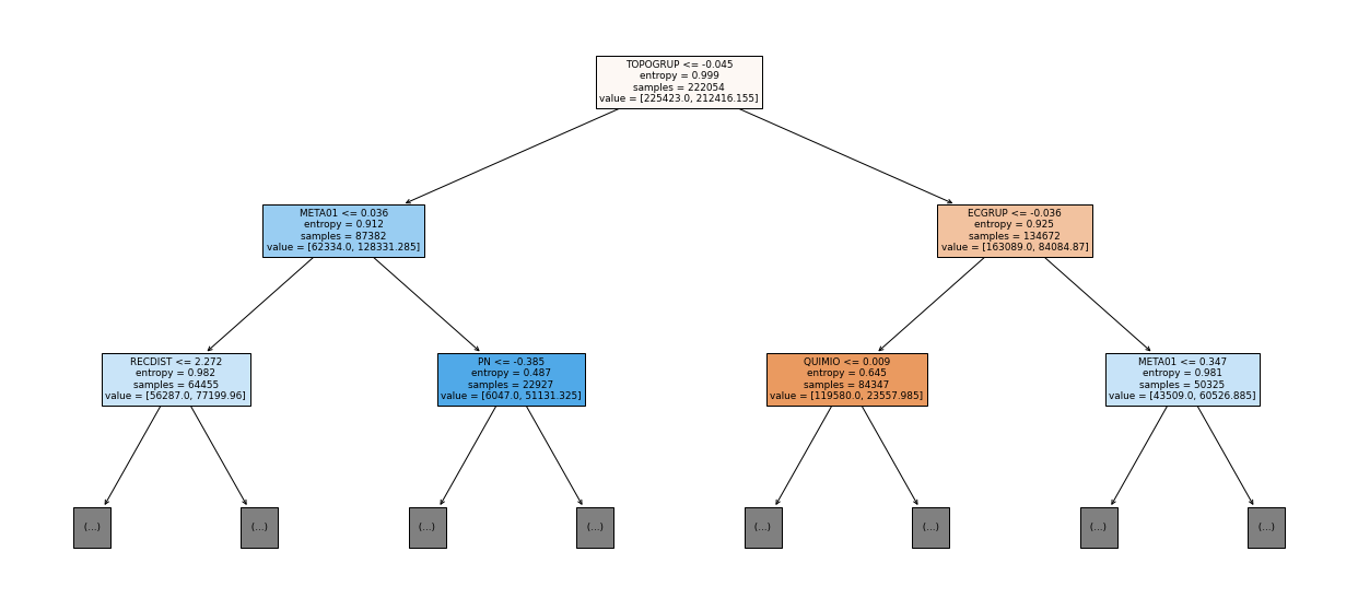
show_tree(rf_sp_00_03, feat_SP_00_03, 2)
[ ]:
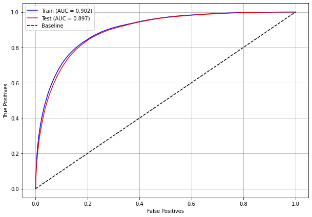
plot_roc_curve(rf_sp_00_03, X_trainSP_00_03, X_testSP_00_03, y_trainSP_00_03, y_testSP_00_03)
[ ]:
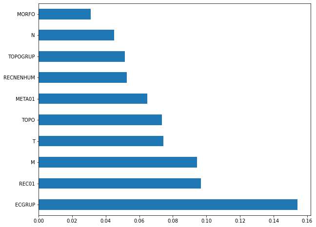
plot_feat_importances(rf_sp_00_03, feat_SP_00_03)
The four most important features in the model were
ECGRUP,REC01,TOPO, andM.
[ ]:
plot_shap_values(rf_sp_00_03, X_testSP_00_03, feat_SP_00_03)
Note that larger values of the ECGRUP column, shown in pink, have more influence for the model’s prediction to be class 1, smaller values have greater weight for the prediction to be class 0. This behavior was expected, because the higher the clinical stage, worse is the stage of cancer.
The other columns shown follow the same logic.
[ ]:
# SP - 2004 to 2007
rf_sp_04_07 = RandomForestClassifier(random_state=seed,
                                     class_weight={0:1, 1:1.33},
                                     criterion='entropy',
                                     max_depth=10)

rf_sp_04_07.fit(X_trainSP_04_07, y_trainSP_04_07)
RandomForestClassifier(class_weight={0: 1, 1: 1.33}, criterion='entropy',
                       max_depth=10, random_state=10)
[ ]:
display_confusion_matrix(rf_sp_04_07, X_testSP_04_07, y_testSP_04_07)

              precision    recall  f1-score   support

           0      0.870     0.822     0.845     12359
           1      0.761     0.822     0.790      8528

    accuracy                          0.822     20887
   macro avg      0.816     0.822     0.818     20887
weighted avg      0.826     0.822     0.823     20887
The confusion matrix obtained for the Random Forest, with SP data from 2004 to 2007, shows a good performance of the model, with 82% of accuracy.
[ ]:
show_tree(rf_sp_04_07, feat_SP_04_07, 2)
[ ]:
plot_roc_curve(rf_sp_04_07, X_trainSP_04_07, X_testSP_04_07, y_trainSP_04_07, y_testSP_04_07)
[ ]:
plot_feat_importances(rf_sp_04_07, feat_SP_04_07)
The four most important features in the model were
ECGRUP,REC01,MandTOPO.
[ ]:
plot_shap_values(rf_sp_04_07, X_testSP_04_07, feat_SP_04_07)
Note that larger values of the ECGRUP column, shown in pink, have more influence for the model’s prediction to be class 1, smaller values have greater weight for the prediction to be class 0. This behavior was expected, because the higher the clinical stage, worse is the stage of cancer.
The other columns shown follow the same logic.
[ ]:
# SP - 2008 to 2011
rf_sp_08_11 = RandomForestClassifier(random_state=seed,
                                     class_weight={0:1, 1:1.5995},
                                     criterion='entropy',
                                     max_depth=10)

rf_sp_08_11.fit(X_trainSP_08_11, y_trainSP_08_11)
RandomForestClassifier(class_weight={0: 1, 1: 1.5995}, criterion='entropy',
                       max_depth=10, random_state=10)
[ ]:
display_confusion_matrix(rf_sp_08_11, X_testSP_08_11, y_testSP_08_11)

              precision    recall  f1-score   support

           0      0.896     0.834     0.864     17549
           1      0.744     0.833     0.786     10194

    accuracy                          0.833     27743
   macro avg      0.820     0.833     0.825     27743
weighted avg      0.840     0.833     0.835     27743
The confusion matrix obtained for the Random Forest, with SP data from 2008 to 2011, shows a good performance of the model, with 83% of accuracy.
[ ]:
show_tree(rf_sp_08_11, feat_SP_08_11, 2)
[ ]:
plot_roc_curve(rf_sp_08_11, X_trainSP_08_11, X_testSP_08_11, y_trainSP_08_11, y_testSP_08_11)
[ ]:
plot_feat_importances(rf_sp_08_11, feat_SP_08_11)
The four most important features in the model were
ECGRUP,REC01,TOPOGRUPandTOPO.
[ ]:
plot_shap_values(rf_sp_08_11, X_testSP_08_11, feat_SP_08_11)
Note that larger values of the ECGRUP column, shown in pink, have more influence for the model’s prediction to be class 1, smaller values have greater weight for the prediction to be class 0. This behavior was expected, because the higher the clinical stage, worse is the stage of cancer.
The other columns shown follow the same logic.
[ ]:
# SP - 2012 to 2015
rf_sp_12_15 = RandomForestClassifier(random_state=seed,
                                     class_weight={0:1, 1:2.218},
                                     criterion='entropy',
                                     max_depth=10)

rf_sp_12_15.fit(X_trainSP_12_15, y_trainSP_12_15)
RandomForestClassifier(class_weight={0: 1, 1: 2.218}, criterion='entropy',
                       max_depth=10, random_state=10)
[ ]:
display_confusion_matrix(rf_sp_12_15, X_testSP_12_15, y_testSP_12_15)

              precision    recall  f1-score   support

           0      0.926     0.841     0.882     24340
           1      0.692     0.842     0.760     10290

    accuracy                          0.842     34630
   macro avg      0.809     0.842     0.821     34630
weighted avg      0.857     0.842     0.846     34630
The confusion matrix obtained for the Random Forest, with SP data from 2012 to 2015, shows a good performance of the model with 84% of accuracy.
[ ]:
show_tree(rf_sp_12_15, feat_SP_12_15, 2)
[ ]:
plot_roc_curve(rf_sp_12_15, X_trainSP_12_15, X_testSP_12_15, y_trainSP_12_15, y_testSP_12_15)
[ ]:
plot_feat_importances(rf_sp_12_15, feat_SP_12_15)
The four most important features in the model were
ECGRUP,M,TOPOandMETA01.
[ ]:
plot_shap_values(rf_sp_12_15, X_testSP_12_15, feat_SP_12_15)
Note that larger values of the ECGRUP column, shown in pink, have more influence for the model’s prediction to be class 1, smaller values have greater weight for the prediction to be class 0. This behavior was expected, because the higher the clinical stage, worse is the stage of cancer.
The other columns shown follow the same logic.
[ ]:
# SP - 2016 to 2021
rf_sp_16_21 = RandomForestClassifier(random_state=seed,
                                     class_weight={0:1, 1:3.362},
                                     criterion='entropy',
                                     max_depth=10)

rf_sp_16_21.fit(X_trainSP_16_21, y_trainSP_16_21)
RandomForestClassifier(class_weight={0: 1, 1: 3.362}, criterion='entropy',
                       max_depth=10, random_state=10)
[ ]:
display_confusion_matrix(rf_sp_16_21, X_testSP_16_21, y_testSP_16_21)

              precision    recall  f1-score   support

           0      0.946     0.831     0.885     20801
           1      0.579     0.830     0.682      5825

    accuracy                          0.831     26626
   macro avg      0.763     0.831     0.784     26626
weighted avg      0.866     0.831     0.840     26626
The confusion matrix obtained for the Random Forest, with SP data from 2016 to 2021, shows a good performance of the model, with 83% of accuracy.
[ ]:
show_tree(rf_sp_16_21, feat_SP_16_21, 2)
[ ]:
plot_roc_curve(rf_sp_16_21, X_trainSP_16_21, X_testSP_16_21, y_trainSP_16_21, y_testSP_16_21)
[ ]:
plot_feat_importances(rf_sp_16_21, feat_SP_16_21)
The four most important features in the model were
ECGRUP,M,META01, andTOPO.
[ ]:
plot_shap_values(rf_sp_16_21, X_testSP_16_21, feat_SP_16_21)
Note that larger values of the ECGRUP column, shown in pink, have more influence for the model’s prediction to be class 1, smaller values have greater weight for the prediction to be class 0. This behavior was expected, because the higher the clinical stage, worse is the stage of cancer.
The other columns shown follow the same logic.
Other states
[ ]:
# Other states - 2000 to 2003
rf_fora_00_03 = RandomForestClassifier(random_state=seed,
                                       class_weight={0:1, 1:1.72},
                                       criterion='entropy',
                                       max_depth=6)

rf_fora_00_03.fit(X_trainOS_00_03, y_trainOS_00_03)
RandomForestClassifier(class_weight={0: 1, 1: 1.72}, criterion='entropy',
                       max_depth=6, random_state=10)
[ ]:
display_confusion_matrix(rf_fora_00_03, X_testOS_00_03, y_testOS_00_03)

              precision    recall  f1-score   support

           0      0.817     0.748     0.781       563
           1      0.662     0.747     0.702       372

    accuracy                          0.748       935
   macro avg      0.740     0.748     0.742       935
weighted avg      0.756     0.748     0.750       935
The confusion matrix obtained for the Random Forest, with other states data from 2000 to 2003, also shows a good performance of the model, and we have a balanced main diagonal with 75% of accuracy.
[ ]:
show_tree(rf_fora_00_03, feat_OS_00_03, 2)
[ ]:
plot_roc_curve(rf_fora_00_03, X_trainOS_00_03, X_testOS_00_03, y_trainOS_00_03, y_testOS_00_03)
[ ]:
plot_feat_importances(rf_fora_00_03, feat_OS_00_03)
The four most important features in the model were
ECGRUP,M,REC01andTOPO.
[ ]:
plot_shap_values(rf_fora_00_03, X_testOS_00_03, feat_OS_00_03)
Note that larger values of the ECGRUP column, shown in pink, have more influence for the model’s prediction to be class 1, smaller values have greater weight for the prediction to be class 0. This behavior was expected, because the higher the clinical stage, worse is the stage of cancer.
The other columns shown follow the same logic.
[ ]:
# Other states - 2004 to 2007
rf_fora_04_07 = RandomForestClassifier(random_state=seed,
                                       class_weight={0:1, 1:1.445},
                                       criterion='entropy',
                                       max_depth=6)

rf_fora_04_07.fit(X_trainOS_04_07, y_trainOS_04_07)
RandomForestClassifier(class_weight={0: 1, 1: 1.445}, criterion='entropy',
                       max_depth=6, random_state=10)
[ ]:
display_confusion_matrix(rf_fora_04_07, X_testOS_04_07, y_testOS_04_07)

              precision    recall  f1-score   support

           0      0.874     0.816     0.844       805
           1      0.737     0.814     0.774       510

    accuracy                          0.815      1315
   macro avg      0.805     0.815     0.809      1315
weighted avg      0.821     0.815     0.817      1315
The confusion matrix obtained for the Random Forest, with other states data from 2004 to 2007, also shows a good performance of the model, with 81% of accuracy.
[ ]:
show_tree(rf_fora_04_07, feat_OS_04_07, 2)
[ ]:
plot_roc_curve(rf_fora_04_07, X_trainOS_04_07, X_testOS_04_07, y_trainOS_04_07, y_testOS_04_07)
[ ]:
plot_feat_importances(rf_fora_04_07, feat_OS_04_07)
The four most important features in the model were
ECGRUP,M,TandTOPO.
[ ]:
plot_shap_values(rf_fora_04_07, X_testOS_04_07, feat_OS_04_07)
Note that larger values of the ECGRUP column, shown in pink, have more influence for the model’s prediction to be class 1, smaller values have greater weight for the prediction to be class 0. This behavior was expected, because the higher the clinical stage, worse is the stage of cancer.
The other columns shown follow the same logic.
[ ]:
# Other states - 2008 to 2011
rf_fora_08_11 = RandomForestClassifier(random_state=seed,
                                       class_weight={0:1, 1:1.75},
                                       criterion='entropy',
                                       max_depth=6)

rf_fora_08_11.fit(X_trainOS_08_11, y_trainOS_08_11)
RandomForestClassifier(class_weight={0: 1, 1: 1.75}, criterion='entropy',
                       max_depth=6, random_state=10)
[ ]:
display_confusion_matrix(rf_fora_08_11, X_testOS_08_11, y_testOS_08_11)

              precision    recall  f1-score   support

           0      0.893     0.811     0.850      1062
           1      0.691     0.813     0.747       552

    accuracy                          0.812      1614
   macro avg      0.792     0.812     0.799      1614
weighted avg      0.824     0.812     0.815      1614
The confusion matrix obtained for the Random Forest, with other states data from 2008 to 2011, also shows a good performance of the model, presenting 81% of accuracy.
[ ]:
show_tree(rf_fora_08_11, feat_OS_08_11, 2)
[ ]:
plot_roc_curve(rf_fora_08_11, X_trainOS_08_11, X_testOS_08_11, y_trainOS_08_11, y_testOS_08_11)
[ ]:
plot_feat_importances(rf_fora_08_11, feat_OS_08_11)
The four most important features in the model were
ECGRUP,M,META01andN.
[ ]:
plot_shap_values(rf_fora_08_11, X_testOS_08_11, feat_OS_08_11)
Note that larger values of the ECGRUP column, shown in pink, have more influence for the model’s prediction to be class 1, smaller values have greater weight for the prediction to be class 0. This behavior was expected, because the higher the clinical stage, worse is the stage of cancer.
The other columns shown follow the same logic.
[ ]:
# Other states - 2012 to 2015
rf_fora_12_15 = RandomForestClassifier(random_state=seed,
                                       class_weight={0:1, 1:2.8},
                                       criterion='entropy',
                                       max_depth=8)

rf_fora_12_15.fit(X_trainOS_12_15, y_trainOS_12_15)
RandomForestClassifier(class_weight={0: 1, 1: 2.8}, criterion='entropy',
                       max_depth=8, random_state=10)
[ ]:
display_confusion_matrix(rf_fora_12_15, X_testOS_12_15, y_testOS_12_15)

              precision    recall  f1-score   support

           0      0.929     0.833     0.879      1563
           1      0.653     0.832     0.732       590

    accuracy                          0.833      2153
   macro avg      0.791     0.833     0.805      2153
weighted avg      0.854     0.833     0.838      2153
The confusion matrix obtained for the Random Forest, with other states data from 2012 to 2015, also shows a good performance of the model, presenting 83% of accuracy.
[ ]:
show_tree(rf_fora_12_15, feat_OS_12_15, 2)
[ ]:
plot_roc_curve(rf_fora_12_15, X_trainOS_12_15, X_testOS_12_15, y_trainOS_12_15, y_testOS_12_15)
[ ]:
plot_feat_importances(rf_fora_12_15, feat_OS_12_15)
The four most important features in the model were
ECGRUP,M,META01andTOPO.
[ ]:
plot_shap_values(rf_fora_12_15, X_testOS_12_15, feat_OS_12_15)
Note that larger values of the ECGRUP column, shown in pink, have more influence for the model’s prediction to be class 1, smaller values have greater weight for the prediction to be class 0. This behavior was expected, because the higher the clinical stage, worse is the stage of cancer.
The other columns shown follow the same logic.
[ ]:
# Other states - 2016 to 2020
rf_fora_16_20 = RandomForestClassifier(random_state=seed,
                                       class_weight={0:1, 1:3.9},
                                       criterion='entropy',
                                       max_depth=8)

rf_fora_16_20.fit(X_trainOS_16_20, y_trainOS_16_20)
RandomForestClassifier(class_weight={0: 1, 1: 3.9}, criterion='entropy',
                       max_depth=8, random_state=10)
[ ]:
display_confusion_matrix(rf_fora_16_20, X_testOS_16_20, y_testOS_16_20)

              precision    recall  f1-score   support

           0      0.942     0.828     0.881      1709
           1      0.584     0.826     0.684       499

    accuracy                          0.827      2208
   macro avg      0.763     0.827     0.783      2208
weighted avg      0.861     0.827     0.837      2208
The confusion matrix obtained for the Random Forest, with other states data from 2016 to 2020, also shows a good performance of the model, presenting 83% of accuracy.
[ ]:
show_tree(rf_fora_16_20, feat_OS_16_20, 2)
[ ]:
plot_roc_curve(rf_fora_16_20, X_trainOS_16_20, X_testOS_16_20, y_trainOS_16_20, y_testOS_16_20)
[ ]:
plot_feat_importances(rf_fora_16_20, feat_OS_16_20)
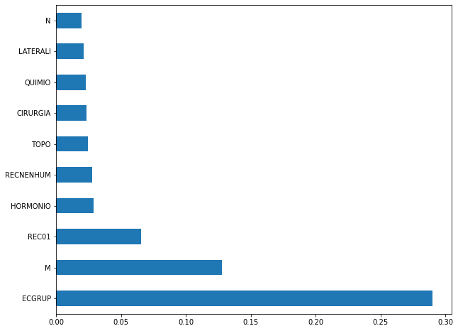
The four most important features in the model were
ECGRUP,M,META01andCIRURGIA.
[ ]:
plot_shap_values(rf_fora_16_20, X_testOS_16_20, feat_OS_16_20)
Note that larger values of the ECGRUP column, shown in pink, have more influence for the model’s prediction to be class 1, smaller values have greater weight for the prediction to be class 0. This behavior was expected, because the higher the clinical stage, worse is the stage of cancer.
The other columns shown follow the same logic.
XGBoost
The training of the XGBoost models follows the same pattern with random_state. The hyperparameter scale_pos_weight was also used in the trainings, in order to obtain a balanced main diagonal in the confusion matrix.
The hyperparameter max_depth was chosen as 10 because the default value for this hyperparameter is 3, a low value for the amount of data we have.
SP
[ ]:
# SP - 2000 to 2003
xgb_sp_00_03 = XGBClassifier(max_depth=8,
                             random_state=seed,
                             scale_pos_weight=1.21)

xgb_sp_00_03.fit(X_trainSP_00_03, y_trainSP_00_03)
XGBClassifier(max_depth=8, random_state=10, scale_pos_weight=1.21)
[ ]:
display_confusion_matrix(xgb_sp_00_03, X_testSP_00_03, y_testSP_00_03)

              precision    recall  f1-score   support

           0      0.847     0.817     0.832      9182
           1      0.783     0.818     0.800      7443

    accuracy                          0.817     16625
   macro avg      0.815     0.817     0.816     16625
weighted avg      0.819     0.817     0.818     16625
The confusion matrix obtained for the XGBoost, with SP data from 2000 to 2003, shows a good performance of the model, here with 82% of accuracy.
[ ]:
plot_roc_curve(xgb_sp_00_03, X_trainSP_00_03, X_testSP_00_03, y_trainSP_00_03, y_testSP_00_03)
[ ]:
plot_feat_importances(xgb_sp_00_03, feat_SP_00_03)
Here we noticed that the most used feature was
ECGRUP, with a lot advantage over the others. Following we haveREC01,MandCIRURGIA.
[ ]:
plot_shap_values(xgb_sp_00_03, X_testSP_00_03, feat_SP_00_03)
Note that larger values of the ECGRUP column, shown in pink, have more influence for the model’s prediction to be class 1, smaller values have greater weight for the prediction to be class 0. This behavior was expected, because the higher the clinical stage, worse is the stage of cancer.
The other columns shown follow the same logic.
[ ]:
# SP - 2004 to 2007
xgb_sp_04_07 = XGBClassifier(max_depth=8,
                             random_state=seed,
                             scale_pos_weight=1.42)

xgb_sp_04_07.fit(X_trainSP_04_07, y_trainSP_04_07)
XGBClassifier(max_depth=8, random_state=10, scale_pos_weight=1.42)
[ ]:
display_confusion_matrix(xgb_sp_04_07, X_testSP_04_07, y_testSP_04_07)

              precision    recall  f1-score   support

           0      0.880     0.835     0.857     12359
           1      0.778     0.834     0.805      8528

    accuracy                          0.835     20887
   macro avg      0.829     0.835     0.831     20887
weighted avg      0.838     0.835     0.836     20887
The confusion matrix obtained for the XGBoost, with SP data from 2004 to 2007, shows a good performance of the model, with 83% of accuracy.
[ ]:
plot_roc_curve(xgb_sp_04_07, X_trainSP_04_07, X_testSP_04_07, y_trainSP_04_07, y_testSP_04_07)

[ ]:
plot_feat_importances(xgb_sp_04_07, feat_SP_04_07)
Here we noticed that the most used feature was
ECGRUP, with a good advantage over the others. Following we haveREC01,META01andCIRURGIA.
[ ]:
plot_shap_values(xgb_sp_04_07, X_testSP_04_07, feat_SP_04_07)
Note that larger values of the ECGRUP column, shown in pink, have more influence for the model’s prediction to be class 1, smaller values have greater weight for the prediction to be class 0. This behavior was expected, because the higher the clinical stage, worse is the stage of cancer.
The other columns shown follow the same logic.
[ ]:
# SP - 2008 to 2011
xgb_sp_08_11 = XGBClassifier(max_depth=8,
                             scale_pos_weight=1.69,
                             random_state=seed)

xgb_sp_08_11.fit(X_trainSP_08_11, y_trainSP_08_11)
XGBClassifier(max_depth=8, random_state=10, scale_pos_weight=1.69)
[ ]:
display_confusion_matrix(xgb_sp_08_11, X_testSP_08_11, y_testSP_08_11)

              precision    recall  f1-score   support

           0      0.905     0.846     0.875     17549
           1      0.762     0.847     0.802     10194

    accuracy                          0.846     27743
   macro avg      0.833     0.847     0.838     27743
weighted avg      0.852     0.846     0.848     27743
The confusion matrix obtained for the XGBoost, with SP data from 2008 to 2011, shows a good performance of the model, with 85% of accuracy.
[ ]:
plot_roc_curve(xgb_sp_08_11, X_trainSP_08_11, X_testSP_08_11, y_trainSP_08_11, y_testSP_08_11)
[ ]:
plot_feat_importances(xgb_sp_08_11, feat_SP_08_11)
Here we noticed that the most used feature was
ECGRUP, with a good advantage over the others. Following we haveREC01,META01andRECNENHUM.
[ ]:
plot_shap_values(xgb_sp_08_11, X_testSP_08_11, feat_SP_08_11)
Note that larger values of the ECGRUP column, shown in pink, have more influence for the model’s prediction to be class 1, smaller values have greater weight for the prediction to be class 0. This behavior was expected, because the higher the clinical stage, worse is the stage of cancer.
The other columns shown follow the same logic.
[ ]:
# SP - 2012 to 2015
xgb_sp_12_15 = XGBClassifier(max_depth=8,
                             random_state=seed,
                             scale_pos_weight=2.18)

xgb_sp_12_15.fit(X_trainSP_12_15, y_trainSP_12_15)
XGBClassifier(max_depth=8, random_state=10, scale_pos_weight=2.18)
[ ]:
display_confusion_matrix(xgb_sp_12_15, X_testSP_12_15, y_testSP_12_15)

              precision    recall  f1-score   support

           0      0.934     0.857     0.893     24340
           1      0.716     0.856     0.780     10290

    accuracy                          0.856     34630
   macro avg      0.825     0.856     0.837     34630
weighted avg      0.869     0.856     0.860     34630
The confusion matrix obtained for the XGBoost, with SP data from 2012 to 2015, shows a good performance of the model, with 86% of accuracy.
[ ]:
plot_roc_curve(xgb_sp_12_15, X_trainSP_12_15, X_testSP_12_15, y_trainSP_12_15, y_testSP_12_15)

[ ]:
plot_feat_importances(xgb_sp_12_15, feat_SP_12_15)
Here we noticed that the most used feature was
ECGRUP, with a good advantage. Following we haveRECNENHUM,CIRURGIAandMETA01.
[ ]:
plot_shap_values(xgb_sp_12_15, X_testSP_12_15, feat_SP_12_15)
Note that larger values of the ECGRUP column, shown in pink, have more influence for the model’s prediction to be class 1, smaller values have greater weight for the prediction to be class 0. This behavior was expected, because the higher the clinical stage, worse is the stage of cancer.
The other columns shown follow the same logic.
[ ]:
# SP - 2016 to 2021
xgb_sp_16_21 = XGBClassifier(max_depth=8,
                             random_state=seed,
                             scale_pos_weight=3.75)

xgb_sp_16_21.fit(X_trainSP_16_21, y_trainSP_16_21)
XGBClassifier(max_depth=8, random_state=10, scale_pos_weight=3.75)
[ ]:
display_confusion_matrix(xgb_sp_16_21, X_testSP_16_21, y_testSP_16_21)
              precision    recall  f1-score   support

           0      0.953     0.850     0.899     20801
           1      0.614     0.851     0.713      5825

    accuracy                          0.850     26626
   macro avg      0.784     0.851     0.806     26626
weighted avg      0.879     0.850     0.858     26626
The confusion matrix obtained for the XGBoost, with SP data from 2016 to 2021, shows a good performance of the model, with 85% of accuracy.
[ ]:
plot_roc_curve(xgb_sp_16_21, X_trainSP_16_21, X_testSP_16_21, y_trainSP_16_21, y_testSP_16_21)

[ ]:
plot_feat_importances(xgb_sp_16_21, feat_SP_16_21)
The four most important features were
ECGRUP,RECNENHUM,GLEASONandRECDIST.
[ ]:
plot_shap_values(xgb_sp_16_21, X_testSP_16_21, feat_SP_16_21)
Note that larger values of the ECGRUP column, shown in pink, have more influence for the model’s prediction to be class 1, smaller values have greater weight for the prediction to be class 0. This behavior was expected, because the higher the clinical stage, worse is the stage of cancer.
The other columns shown follow the same logic.
Other states
[ ]:
# Other states - 2000 to 2003
xgb_fora_00_03 = XGBClassifier(max_depth=5,
                               scale_pos_weight=1.67,
                               random_state=seed)

xgb_fora_00_03.fit(X_trainOS_00_03, y_trainOS_00_03)
XGBClassifier(max_depth=5, random_state=10, scale_pos_weight=1.67)
[ ]:
display_confusion_matrix(xgb_fora_00_03, X_testOS_00_03, y_testOS_00_03)

              precision    recall  f1-score   support

           0      0.822     0.753     0.786       563
           1      0.668     0.753     0.708       372

    accuracy                          0.753       935
   macro avg      0.745     0.753     0.747       935
weighted avg      0.761     0.753     0.755       935
The confusion matrix obtained for the XGBoost, with other states data from 2000 to 2003, also shows a good performance of the model, with 75% of accuracy.
[ ]:
plot_roc_curve(xgb_fora_00_03, X_trainOS_00_03, X_testOS_00_03, y_trainOS_00_03, y_testOS_00_03)
[ ]:
plot_feat_importances(xgb_fora_00_03, feat_OS_00_03)
Again we noticed that the most used feature was
ECGRUP, with a good advantage. The following most important features wereREC01,MandMETA01.
[ ]:
plot_shap_values(xgb_fora_00_03, X_testOS_00_03, feat_OS_00_03)
Note that larger values of the ECGRUP column, shown in pink, have more influence for the model’s prediction to be class 1, smaller values have greater weight for the prediction to be class 0. This behavior was expected, because the higher the clinical stage, worse is the stage of cancer.
The other columns shown follow the same logic.
[ ]:
# Other states - 2004 to 2007
xgb_fora_04_07 = XGBClassifier(max_depth=5,
                               scale_pos_weight=1.345,
                               random_state=seed)

xgb_fora_04_07.fit(X_trainOS_04_07, y_trainOS_04_07)
XGBClassifier(max_depth=5, random_state=10, scale_pos_weight=1.345)
[ ]:
display_confusion_matrix(xgb_fora_04_07, X_testOS_04_07, y_testOS_04_07)

              precision    recall  f1-score   support

           0      0.890     0.836     0.862       805
           1      0.764     0.837     0.799       510

    accuracy                          0.837      1315
   macro avg      0.827     0.837     0.831      1315
weighted avg      0.841     0.837     0.838      1315
The confusion matrix obtained for the XGBoost, with other states data from 2004 to 2007, also shows a good performance of the model with 84% of accuracy.
[ ]:
plot_roc_curve(xgb_fora_04_07, X_trainOS_04_07, X_testOS_04_07, y_trainOS_04_07, y_testOS_04_07)
[ ]:
plot_feat_importances(xgb_fora_04_07, feat_OS_04_07)
Again we noticed that the most used feature was
ECGRUP, with a good advantage. The following most important features wereREC01,TandMETA01.
[ ]:
plot_shap_values(xgb_fora_04_07, X_testOS_04_07, feat_OS_04_07)
Note that larger values of the ECGRUP column, shown in pink, have more influence for the model’s prediction to be class 1, smaller values have greater weight for the prediction to be class 0. This behavior was expected, because the higher the clinical stage, worse is the stage of cancer.
The other columns shown follow the same logic.
[ ]:
# Other states - 2008 to 2011
xgb_fora_08_11 = XGBClassifier(max_depth=5,
                               scale_pos_weight=1.65,
                               random_state=seed)

xgb_fora_08_11.fit(X_trainOS_08_11, y_trainOS_08_11)
XGBClassifier(max_depth=5, random_state=10, scale_pos_weight=1.65)
[ ]:
display_confusion_matrix(xgb_fora_08_11, X_testOS_08_11, y_testOS_08_11)

              precision    recall  f1-score   support

           0      0.904     0.831     0.866      1062
           1      0.718     0.830     0.770       552

    accuracy                          0.830      1614
   macro avg      0.811     0.830     0.818      1614
weighted avg      0.840     0.830     0.833      1614
The confusion matrix obtained for the XGBoost, with other states data from 2008 to 2011, also shows a good performance of the model with 83% of accuracy.
[ ]:
plot_roc_curve(xgb_fora_08_11, X_trainOS_08_11, X_testOS_08_11, y_trainOS_08_11, y_testOS_08_11)
[ ]:
plot_feat_importances(xgb_fora_08_11, feat_OS_08_11)
Again we noticed that the most used feature was
ECGRUP, but not with a lot of advantage. The following most important features wereM,REC01andHORMONIO.
[ ]:
plot_shap_values(xgb_fora_08_11, X_testOS_08_11, feat_OS_08_11)
Note that larger values of the ECGRUP column, shown in pink, have more influence for the model’s prediction to be class 1, smaller values have greater weight for the prediction to be class 0. This behavior was expected, because the higher the clinical stage, worse is the stage of cancer.
The other columns shown follow the same logic.
[ ]:
# Other states - 2012 to 2015
xgb_fora_12_15 = XGBClassifier(max_depth=5,
                               scale_pos_weight=2.7,
                               random_state=seed)

xgb_fora_12_15.fit(X_trainOS_12_15, y_trainOS_12_15)
XGBClassifier(max_depth=5, random_state=10, scale_pos_weight=2.7)
[ ]:
display_confusion_matrix(xgb_fora_12_15, X_testOS_12_15, y_testOS_12_15)

              precision    recall  f1-score   support

           0      0.932     0.837     0.882      1563
           1      0.660     0.837     0.738       590

    accuracy                          0.837      2153
   macro avg      0.796     0.837     0.810      2153
weighted avg      0.857     0.837     0.842      2153
The confusion matrix obtained for the XGBoost, with other states data from 2012 to 2015, also shows a good performance of the model with 84% of accuracy.
[ ]:
plot_roc_curve(xgb_fora_12_15, X_trainOS_12_15, X_testOS_12_15, y_trainOS_12_15, y_testOS_12_15)
[ ]:
plot_feat_importances(xgb_fora_12_15, feat_OS_12_15)
The four most important features were
ECGRUP,M,REC01andRECLOCAL.
[ ]:
plot_shap_values(xgb_fora_12_15, X_testOS_12_15, feat_OS_12_15)
Note that larger values of the ECGRUP column, shown in pink, have more influence for the model’s prediction to be class 1, smaller values have greater weight for the prediction to be class 0. This behavior was expected, because the higher the clinical stage, worse is the stage of cancer.
The other columns shown follow the same logic.
[ ]:
# Other states - 2016 to 2020
xgb_fora_16_20 = XGBClassifier(max_depth=5,
                               scale_pos_weight=4.5,
                               random_state=seed)

xgb_fora_16_20.fit(X_trainOS_16_20, y_trainOS_16_20)
XGBClassifier(max_depth=5, random_state=10, scale_pos_weight=4.5)
[ ]:
display_confusion_matrix(xgb_fora_16_20, X_testOS_16_20, y_testOS_16_20)

              precision    recall  f1-score   support

           0      0.949     0.844     0.893      1709
           1      0.612     0.846     0.710       499

    accuracy                          0.844      2208
   macro avg      0.781     0.845     0.802      2208
weighted avg      0.873     0.844     0.852      2208
The confusion matrix obtained for the XGBoost, with other states data from 2016 to 2020, shows the best performance comparing with the other models, with 84% of accuracy.
[ ]:
plot_roc_curve(xgb_fora_16_20, X_trainOS_16_20, X_testOS_16_20, y_trainOS_16_20, y_testOS_16_20)
[ ]:
plot_feat_importances(xgb_fora_16_20, feat_OS_16_20)
The four most important features were
ECGRUP,RECNENHUM,CIRURGIAandGLEASON.
[ ]:
plot_shap_values(xgb_fora_16_20, X_testOS_16_20, feat_OS_16_20)
Note that larger values of the ECGRUP column, shown in pink, have more influence for the model’s prediction to be class 1, smaller values have greater weight for the prediction to be class 0. This behavior was expected, because the higher the clinical stage, worse is the stage of cancer.
The other columns shown follow the same logic.
Testing models with data from other years
We will use test data from the following years in the trained models for each set of years grouped together.
Random Forest SP for years 2000 to 2003
[ ]:
display_confusion_matrix(rf_sp_00_03, X_testSP_04_07, y_testSP_04_07)

              precision    recall  f1-score   support

           0      0.873     0.813     0.842     12359
           1      0.753     0.829     0.789      8528

    accuracy                          0.819     20887
   macro avg      0.813     0.821     0.815     20887
weighted avg      0.824     0.819     0.820     20887
[ ]:
display_confusion_matrix(rf_sp_00_03, X_testSP_08_11, y_testSP_08_11)

              precision    recall  f1-score   support

           0      0.898     0.808     0.851     17549
           1      0.718     0.842     0.775     10194

    accuracy                          0.821     27743
   macro avg      0.808     0.825     0.813     27743
weighted avg      0.832     0.821     0.823     27743
[ ]:
display_confusion_matrix(rf_sp_00_03, X_testSP_12_15, y_testSP_12_15)
              precision    recall  f1-score   support

           0      0.936     0.794     0.859     24340
           1      0.641     0.872     0.739     10290

    accuracy                          0.817     34630
   macro avg      0.788     0.833     0.799     34630
weighted avg      0.848     0.817     0.823     34630
[ ]:
display_confusion_matrix(rf_sp_00_03, X_testSP_16_21, y_testSP_16_21)

              precision    recall  f1-score   support

           0      0.970     0.648     0.777     20801
           1      0.425     0.929     0.583      5825

    accuracy                          0.709     26626
   macro avg      0.697     0.788     0.680     26626
weighted avg      0.851     0.709     0.734     26626
XGBoost SP for years 2000 to 2003
[ ]:
display_confusion_matrix(xgb_sp_00_03, X_testSP_04_07, y_testSP_04_07)

              precision    recall  f1-score   support

           0      0.852     0.844     0.848     12359
           1      0.777     0.787     0.782      8528

    accuracy                          0.821     20887
   macro avg      0.814     0.816     0.815     20887
weighted avg      0.821     0.821     0.821     20887
[ ]:
display_confusion_matrix(xgb_sp_00_03, X_testSP_08_11, y_testSP_08_11)

              precision    recall  f1-score   support

           0      0.876     0.845     0.860     17549
           1      0.749     0.795     0.771     10194

    accuracy                          0.827     27743
   macro avg      0.813     0.820     0.816     27743
weighted avg      0.830     0.827     0.828     27743
[ ]:
display_confusion_matrix(xgb_sp_00_03, X_testSP_12_15, y_testSP_12_15)
              precision    recall  f1-score   support

           0      0.912     0.834     0.871     24340
           1      0.674     0.810     0.735     10290

    accuracy                          0.827     34630
   macro avg      0.793     0.822     0.803     34630
weighted avg      0.841     0.827     0.831     34630
[ ]:
display_confusion_matrix(xgb_sp_00_03, X_testSP_16_21, y_testSP_16_21)
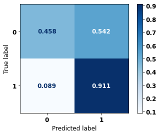
              precision    recall  f1-score   support

           0      0.948     0.458     0.618     20801
           1      0.320     0.911     0.474      5825

    accuracy                          0.558     26626
   macro avg      0.634     0.685     0.546     26626
weighted avg      0.811     0.558     0.587     26626
Random Forest SP for years 2004 to 2007
[ ]:
display_confusion_matrix(rf_sp_04_07, X_testSP_08_11, y_testSP_08_11)

              precision    recall  f1-score   support

           0      0.895     0.825     0.858     17549
           1      0.734     0.833     0.780     10194

    accuracy                          0.828     27743
   macro avg      0.814     0.829     0.819     27743
weighted avg      0.836     0.828     0.830     27743
[ ]:
display_confusion_matrix(rf_sp_04_07, X_testSP_12_15, y_testSP_12_15)

              precision    recall  f1-score   support

           0      0.930     0.816     0.869     24340
           1      0.663     0.854     0.746     10290

    accuracy                          0.827     34630
   macro avg      0.796     0.835     0.808     34630
weighted avg      0.850     0.827     0.833     34630
[ ]:
display_confusion_matrix(rf_sp_04_07, X_testSP_16_21, y_testSP_16_21)
              precision    recall  f1-score   support

           0      0.963     0.694     0.807     20801
           1      0.453     0.906     0.604      5825

    accuracy                          0.740     26626
   macro avg      0.708     0.800     0.705     26626
weighted avg      0.852     0.740     0.762     26626
XGBoost SP for years 2004 to 2007
[ ]:
display_confusion_matrix(xgb_sp_04_07, X_testSP_08_11, y_testSP_08_11)

              precision    recall  f1-score   support

           0      0.891     0.842     0.866     17549
           1      0.752     0.823     0.786     10194

    accuracy                          0.835     27743
   macro avg      0.821     0.833     0.826     27743
weighted avg      0.840     0.835     0.836     27743
[ ]:
display_confusion_matrix(xgb_sp_04_07, X_testSP_12_15, y_testSP_12_15)
              precision    recall  f1-score   support

           0      0.905     0.840     0.871     24340
           1      0.677     0.792     0.730     10290

    accuracy                          0.826     34630
   macro avg      0.791     0.816     0.801     34630
weighted avg      0.837     0.826     0.829     34630
[ ]:
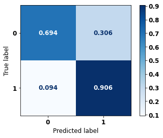
display_confusion_matrix(xgb_sp_04_07, X_testSP_16_21, y_testSP_16_21)

              precision    recall  f1-score   support

           0      0.932     0.619     0.744     20801
           1      0.381     0.839     0.524      5825

    accuracy                          0.667     26626
   macro avg      0.657     0.729     0.634     26626
weighted avg      0.812     0.667     0.696     26626
Random Forest SP for years 2008 to 2011
[ ]:
display_confusion_matrix(rf_sp_08_11, X_testSP_12_15, y_testSP_12_15)
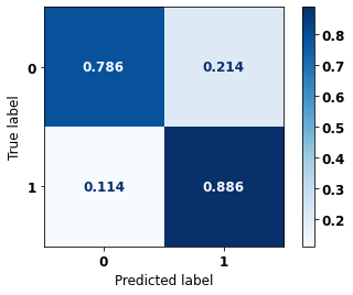
              precision    recall  f1-score   support

           0      0.942     0.786     0.857     24340
           1      0.636     0.886     0.741     10290

    accuracy                          0.816     34630
   macro avg      0.789     0.836     0.799     34630
weighted avg      0.851     0.816     0.822     34630
[ ]:
display_confusion_matrix(rf_sp_08_11, X_testSP_16_21, y_testSP_16_21)
              precision    recall  f1-score   support

           0      0.972     0.647     0.777     20801
           1      0.425     0.933     0.584      5825

    accuracy                          0.709     26626
   macro avg      0.698     0.790     0.680     26626
weighted avg      0.852     0.709     0.734     26626
XGBoost SP for years 2008 to 2011
[ ]:
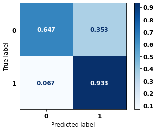
display_confusion_matrix(xgb_sp_08_11, X_testSP_12_15, y_testSP_12_15)
              precision    recall  f1-score   support

           0      0.924     0.502     0.651     24340
           1      0.434     0.902     0.586     10290

    accuracy                          0.621     34630
   macro avg      0.679     0.702     0.618     34630
weighted avg      0.778     0.621     0.631     34630
[ ]:
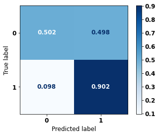
display_confusion_matrix(xgb_sp_08_11, X_testSP_16_21, y_testSP_16_21)
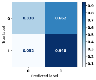
              precision    recall  f1-score   support

           0      0.959     0.338     0.500     20801
           1      0.286     0.948     0.440      5825

    accuracy                          0.472     26626
   macro avg      0.622     0.643     0.470     26626
weighted avg      0.812     0.472     0.487     26626
Random Forest SP for years 2012 to 2015
[ ]:
display_confusion_matrix(rf_sp_12_15, X_testSP_16_21, y_testSP_16_21)

              precision    recall  f1-score   support

           0      0.951     0.784     0.860     20801
           1      0.527     0.856     0.652      5825

    accuracy                          0.800     26626
   macro avg      0.739     0.820     0.756     26626
weighted avg      0.858     0.800     0.814     26626
XGBoost SP for years 2012 to 2015
[ ]:
display_confusion_matrix(xgb_sp_12_15, X_testSP_16_21, y_testSP_16_21)

              precision    recall  f1-score   support

           0      0.948     0.808     0.872     20801
           1      0.551     0.841     0.666      5825

    accuracy                          0.815     26626
   macro avg      0.749     0.824     0.769     26626
weighted avg      0.861     0.815     0.827     26626
Random Forest Other states for years 2000 to 2003
[ ]:
display_confusion_matrix(rf_fora_00_03, X_testOS_04_07, y_testOS_04_07)
              precision    recall  f1-score   support

           0      0.890     0.798     0.841       805
           1      0.726     0.845     0.781       510

    accuracy                          0.816      1315
   macro avg      0.808     0.821     0.811      1315
weighted avg      0.826     0.816     0.818      1315
[ ]:
display_confusion_matrix(rf_fora_00_03, X_testOS_08_11, y_testOS_08_11)

              precision    recall  f1-score   support

           0      0.922     0.754     0.830      1062
           1      0.650     0.877     0.746       552

    accuracy                          0.796      1614
   macro avg      0.786     0.816     0.788      1614
weighted avg      0.829     0.796     0.801      1614
[ ]:
display_confusion_matrix(rf_fora_00_03, X_testOS_12_15, y_testOS_12_15)
              precision    recall  f1-score   support

           0      0.950     0.739     0.831      1563
           1      0.565     0.897     0.693       590

    accuracy                          0.782      2153
   macro avg      0.757     0.818     0.762      2153
weighted avg      0.844     0.782     0.793      2153
[ ]:
display_confusion_matrix(rf_fora_00_03, X_testOS_16_20, y_testOS_16_20)

              precision    recall  f1-score   support

           0      0.963     0.702     0.812      1709
           1      0.470     0.908     0.620       499

    accuracy                          0.748      2208
   macro avg      0.717     0.805     0.716      2208
weighted avg      0.852     0.748     0.768      2208
XGBoost Other states for years 2000 to 2003
[ ]:
display_confusion_matrix(xgb_fora_00_03, X_testOS_04_07, y_testOS_04_07)
              precision    recall  f1-score   support

           0      0.886     0.831     0.858       805
           1      0.757     0.831     0.793       510

    accuracy                          0.831      1315
   macro avg      0.822     0.831     0.825      1315
weighted avg      0.836     0.831     0.832      1315
[ ]:
display_confusion_matrix(xgb_fora_00_03, X_testOS_08_11, y_testOS_08_11)

              precision    recall  f1-score   support

           0      0.914     0.786     0.845      1062
           1      0.676     0.857     0.756       552

    accuracy                          0.810      1614
   macro avg      0.795     0.822     0.800      1614
weighted avg      0.832     0.810     0.815      1614
[ ]:
display_confusion_matrix(xgb_fora_00_03, X_testOS_12_15, y_testOS_12_15)

              precision    recall  f1-score   support

           0      0.944     0.770     0.848      1563
           1      0.591     0.880     0.707       590

    accuracy                          0.800      2153
   macro avg      0.768     0.825     0.778      2153
weighted avg      0.848     0.800     0.810      2153
[ ]:
display_confusion_matrix(xgb_fora_00_03, X_testOS_16_20, y_testOS_16_20)

              precision    recall  f1-score   support

           0      0.956     0.726     0.825      1709
           1      0.486     0.886     0.627       499

    accuracy                          0.762      2208
   macro avg      0.721     0.806     0.726      2208
weighted avg      0.850     0.762     0.781      2208
Random Forest Other states for years 2004 to 2007
[ ]:
display_confusion_matrix(rf_fora_04_07, X_testOS_08_11, y_testOS_08_11)

              precision    recall  f1-score   support

           0      0.901     0.791     0.843      1062
           1      0.674     0.833     0.746       552

    accuracy                          0.805      1614
   macro avg      0.788     0.812     0.794      1614
weighted avg      0.824     0.805     0.809      1614
[ ]:
display_confusion_matrix(rf_fora_04_07, X_testOS_12_15, y_testOS_12_15)
              precision    recall  f1-score   support

           0      0.946     0.751     0.837      1563
           1      0.573     0.886     0.696       590

    accuracy                          0.788      2153
   macro avg      0.760     0.819     0.767      2153
weighted avg      0.844     0.788     0.799      2153
[ ]:
display_confusion_matrix(rf_fora_04_07, X_testOS_16_20, y_testOS_16_20)

              precision    recall  f1-score   support

           0      0.962     0.714     0.820      1709
           1      0.480     0.904     0.627       499

    accuracy                          0.757      2208
   macro avg      0.721     0.809     0.723      2208
weighted avg      0.853     0.757     0.776      2208
XGBoost Other states for years 2004 to 2007
[ ]:
display_confusion_matrix(xgb_fora_04_07, X_testOS_08_11, y_testOS_08_11)

              precision    recall  f1-score   support

           0      0.909     0.812     0.858      1062
           1      0.700     0.844     0.765       552

    accuracy                          0.823      1614
   macro avg      0.804     0.828     0.811      1614
weighted avg      0.838     0.823     0.826      1614
[ ]:
display_confusion_matrix(xgb_fora_04_07, X_testOS_12_15, y_testOS_12_15)

              precision    recall  f1-score   support

           0      0.945     0.771     0.849      1563
           1      0.592     0.881     0.708       590

    accuracy                          0.801      2153
   macro avg      0.769     0.826     0.779      2153
weighted avg      0.848     0.801     0.811      2153
[ ]:
display_confusion_matrix(xgb_fora_04_07, X_testOS_16_20, y_testOS_16_20)

              precision    recall  f1-score   support

           0      0.947     0.748     0.836      1709
           1      0.498     0.856     0.630       499

    accuracy                          0.773      2208
   macro avg      0.722     0.802     0.733      2208
weighted avg      0.845     0.773     0.789      2208
Random Forest Other states for years 2008 to 2011
[ ]:
display_confusion_matrix(rf_fora_08_11, X_testOS_12_15, y_testOS_12_15)
              precision    recall  f1-score   support

           0      0.936     0.793     0.858      1563
           1      0.609     0.856     0.712       590

    accuracy                          0.810      2153
   macro avg      0.772     0.824     0.785      2153
weighted avg      0.846     0.810     0.818      2153
[ ]:
display_confusion_matrix(rf_fora_08_11, X_testOS_16_20, y_testOS_16_20)

              precision    recall  f1-score   support

           0      0.954     0.761     0.846      1709
           1      0.516     0.874     0.649       499

    accuracy                          0.786      2208
   macro avg      0.735     0.817     0.748      2208
weighted avg      0.855     0.786     0.802      2208
XGBoost Other states for years 2008 to 2011
[ ]:
display_confusion_matrix(xgb_fora_08_11, X_testOS_12_15, y_testOS_12_15)

              precision    recall  f1-score   support

           0      0.928     0.811     0.866      1563
           1      0.625     0.832     0.714       590

    accuracy                          0.817      2153
   macro avg      0.776     0.822     0.790      2153
weighted avg      0.845     0.817     0.824      2153
[ ]:
display_confusion_matrix(xgb_fora_08_11, X_testOS_16_20, y_testOS_16_20)

              precision    recall  f1-score   support

           0      0.939     0.796     0.861      1709
           1      0.540     0.822     0.652       499

    accuracy                          0.802      2208
   macro avg      0.739     0.809     0.757      2208
weighted avg      0.849     0.802     0.814      2208
Random Forest Other states for years 2012 to 2015
[ ]:
display_confusion_matrix(rf_fora_12_15, X_testOS_16_20, y_testOS_16_20)

              precision    recall  f1-score   support

           0      0.952     0.791     0.864      1709
           1      0.546     0.864     0.669       499

    accuracy                          0.807      2208
   macro avg      0.749     0.827     0.767      2208
weighted avg      0.860     0.807     0.820      2208
XGBoost Other states for years 2012 to 2015
[ ]:
display_confusion_matrix(xgb_fora_12_15, X_testOS_16_20, y_testOS_16_20)

              precision    recall  f1-score   support

           0      0.949     0.804     0.870      1709
           1      0.559     0.852     0.675       499

    accuracy                          0.815      2208
   macro avg      0.754     0.828     0.773      2208
weighted avg      0.861     0.815     0.826      2208
Fourth approach
Approach with grouped years, using only morphologies with final digit equal to 3 and without the column EC.
Preprocessing
Now we are going to divide the data into training and testing, and then do the preprocessing in both datasets to perform the training of the models and their evaluation. We will use the years grouped too, resulting in 5 datasets for SP and more 5 for other states.
First, it is necessary to define the columns that will be used as features and the label. We will not use some columns of the data: UFRESID, because we already have the division between SP and other states in the two datasets.
It was chosen to keep the column IDADE, so we will not use the FAIXAETAR, as well as the column ECGRUP and not the column EC. Finally, the other columns contained in the list list_drop are possible labels, so they will not be used as features for machine learning models.
[ ]:
list_drop = ['UFRESID', 'FAIXAETAR', 'ULTICONS', 'ULTIDIAG', 'ULTITRAT',
             'vivo_ano1', 'vivo_ano3', 'vivo_ano5', 'ULTINFO', 'EC', 'obito_geral']

lb = 'obito_cancer'
A function was created to perform the preprocessing, preprocessing, that uses the other functions created, get_train_test (divides the dataset into train and test sets), train_preprocessing (do the preprocessing of the train set) and test_preprocessing (do the preprocessing of the test set).
The process will be done 5 times for SP and other states, using the datasets with grouped years.
To see the complete function go to the functions section.
SP
[ ]:
X_trainSP_00_03, X_testSP_00_03, y_trainSP_00_03, y_testSP_00_03, feat_SP_00_03 = preprocessing(df_SP, list_drop, lb,
                                                                                                group_years=True, first_year=2000,
                                                                                                last_year=2003, morpho3=True,
                                                                                                random_state=seed,
                                                                                                balance_data=False,
                                                                                                encoder_type='LabelEncoder',
                                                                                                norm_name='StandardScaler')
X_train = (46098, 65), X_test = (15367, 65)
y_train = (46098,), y_test = (15367,)
[ ]:
X_trainSP_04_07, X_testSP_04_07, y_trainSP_04_07, y_testSP_04_07, feat_SP_04_07 = preprocessing(df_SP, list_drop, lb,
                                                                                                group_years=True, first_year=2004,
                                                                                                last_year=2007, morpho3=True,
                                                                                                random_state=seed,
                                                                                                balance_data=False,
                                                                                                encoder_type='LabelEncoder',
                                                                                                norm_name='StandardScaler')
X_train = (58169, 65), X_test = (19390, 65)
y_train = (58169,), y_test = (19390,)
[ ]:
X_trainSP_08_11, X_testSP_08_11, y_trainSP_08_11, y_testSP_08_11, feat_SP_08_11 = preprocessing(df_SP, list_drop, lb,
                                                                                                group_years=True, first_year=2008,
                                                                                                last_year=2011, morpho3=True,
                                                                                                random_state=seed,
                                                                                                balance_data=False,
                                                                                                encoder_type='LabelEncoder',
                                                                                                norm_name='StandardScaler')
X_train = (77412, 65), X_test = (25804, 65)
y_train = (77412,), y_test = (25804,)
[ ]:
X_trainSP_12_15, X_testSP_12_15, y_trainSP_12_15, y_testSP_12_15, feat_SP_12_15 = preprocessing(df_SP, list_drop, lb,
                                                                                                group_years=True, first_year=2012,
                                                                                                last_year=2015, morpho3=True,
                                                                                                random_state=seed,
                                                                                                balance_data=False,
                                                                                                encoder_type='LabelEncoder',
                                                                                                norm_name='StandardScaler')
X_train = (96124, 65), X_test = (32042, 65)
y_train = (96124,), y_test = (32042,)
[ ]:
X_trainSP_16_21, X_testSP_16_21, y_trainSP_16_21, y_testSP_16_21, feat_SP_16_21 = preprocessing(df_SP, list_drop, lb,
                                                                                                group_years=True, first_year=2016,
                                                                                                last_year=2021, morpho3=True,
                                                                                                random_state=seed,
                                                                                                balance_data=False,
                                                                                                encoder_type='LabelEncoder',
                                                                                                norm_name='StandardScaler')
X_train = (73682, 65), X_test = (24561, 65)
y_train = (73682,), y_test = (24561,)
Other states
[ ]:
X_trainOS_00_03, X_testOS_00_03, y_trainOS_00_03, y_testOS_00_03, feat_OS_00_03 = preprocessing(df_fora, list_drop, lb,
                                                                                                group_years=True, first_year=2000,
                                                                                                last_year=2003, morpho3=True,
                                                                                                random_state=seed,
                                                                                                balance_data=False,
                                                                                                encoder_type='LabelEncoder',
                                                                                                norm_name='StandardScaler')
X_train = (2592, 65), X_test = (865, 65)
y_train = (2592,), y_test = (865,)
[ ]:
X_trainOS_04_07, X_testOS_04_07, y_trainOS_04_07, y_testOS_04_07, feat_OS_04_07 = preprocessing(df_fora, list_drop, lb,
                                                                                                group_years=True, first_year=2004,
                                                                                                last_year=2007, morpho3=True,
                                                                                                random_state=seed,
                                                                                                balance_data=False,
                                                                                                encoder_type='LabelEncoder',
                                                                                                norm_name='StandardScaler')
X_train = (3694, 65), X_test = (1232, 65)
y_train = (3694,), y_test = (1232,)
[ ]:
X_trainOS_08_11, X_testOS_08_11, y_trainOS_08_11, y_testOS_08_11, feat_OS_08_11 = preprocessing(df_fora, list_drop, lb,
                                                                                                group_years=True, first_year=2008,
                                                                                                last_year=2011, morpho3=True,
                                                                                                random_state=seed,
                                                                                                balance_data=False,
                                                                                                encoder_type='LabelEncoder',
                                                                                                norm_name='StandardScaler')
X_train = (4536, 65), X_test = (1513, 65)
y_train = (4536,), y_test = (1513,)
[ ]:
X_trainOS_12_15, X_testOS_12_15, y_trainOS_12_15, y_testOS_12_15, feat_OS_12_15 = preprocessing(df_fora, list_drop, lb,
                                                                                                group_years=True, first_year=2012,
                                                                                                last_year=2015, morpho3=True,
                                                                                                random_state=seed,
                                                                                                balance_data=False,
                                                                                                encoder_type='LabelEncoder',
                                                                                                norm_name='StandardScaler')
X_train = (6069, 65), X_test = (2024, 65)
y_train = (6069,), y_test = (2024,)
[ ]:
X_trainOS_16_20, X_testOS_16_20, y_trainOS_16_20, y_testOS_16_20, feat_OS_16_20 = preprocessing(df_fora, list_drop, lb,
                                                                                                group_years=True, first_year=2016,
                                                                                                last_year=2020, morpho3=True,
                                                                                                random_state=seed,
                                                                                                balance_data=False,
                                                                                                encoder_type='LabelEncoder',
                                                                                                norm_name='StandardScaler')
X_train = (6185, 65), X_test = (2062, 65)
y_train = (6185,), y_test = (2062,)
Training and evaluation of the models
After dividing the data into training and testing, using the encoder and normalizing, the data is ready to be used by the machine learning models.
Random Forest
The first model is the Random Forest, the random_state will be used as a parameter, to obtain the same training values of the model every time it is runned.
The hyperparameter class_weight was used because the models have difficulty to learn the class with fewer examples.
SP
[ ]:
# SP - 2000 to 2003
rf_sp_00_03 = RandomForestClassifier(random_state=seed,
                                     class_weight={0:1, 1:1},
                                     criterion='entropy',
                                     max_depth=10)

rf_sp_00_03.fit(X_trainSP_00_03, y_trainSP_00_03)
RandomForestClassifier(class_weight={0: 1, 1: 1}, criterion='entropy',
                       max_depth=10, random_state=10)
[ ]:
display_confusion_matrix(rf_sp_00_03, X_testSP_00_03, y_testSP_00_03)
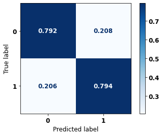
              precision    recall  f1-score   support

           0      0.805     0.792     0.799      7965
           1      0.780     0.794     0.787      7402

    accuracy                          0.793     15367
   macro avg      0.793     0.793     0.793     15367
weighted avg      0.793     0.793     0.793     15367
The confusion matrix obtained for the Random Forest, with SP data from 2000 to 2003, shows a good performance of the model, with 79% of accuracy.
[ ]:
show_tree(rf_sp_00_03, feat_SP_00_03, 2)
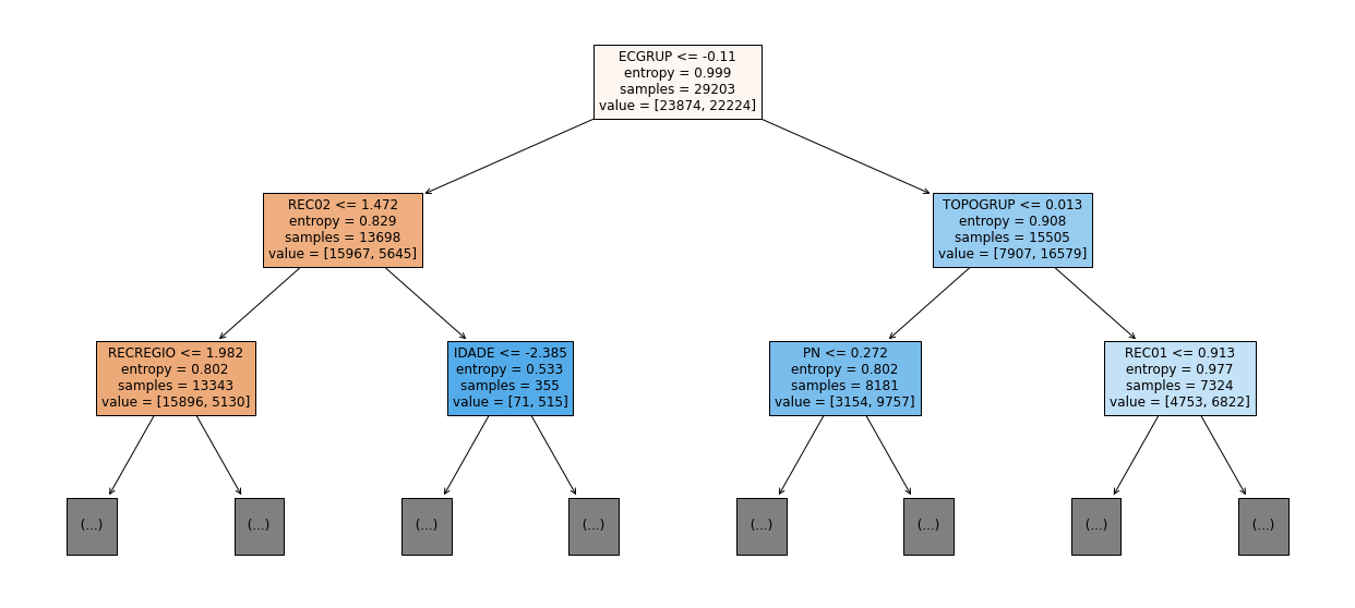
[ ]:
plot_roc_curve(rf_sp_00_03, X_trainSP_00_03, X_testSP_00_03, y_trainSP_00_03, y_testSP_00_03)
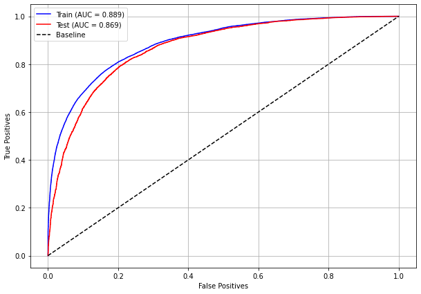
[ ]:
plot_feat_importances(rf_sp_00_03, feat_SP_00_03)
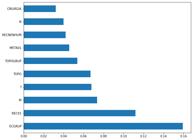
The four most important features in the model were
ECGRUP,REC01,M, andT.
[ ]:
plot_shap_values(rf_sp_00_03, X_testSP_00_03, feat_SP_00_03)
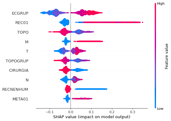
Note that larger values of the ECGRUP column, shown in pink, have more influence for the model’s prediction to be class 1, smaller values have greater weight for the prediction to be class 0. This behavior was expected, because the higher the clinical stage, worse is the stage of cancer.
The other columns shown follow the same logic.
[ ]:
# SP - 2004 to 2007
rf_sp_04_07 = RandomForestClassifier(random_state=seed,
                                     class_weight={0:1, 1:1.2},
                                     criterion='entropy',
                                     max_depth=10)

rf_sp_04_07.fit(X_trainSP_04_07, y_trainSP_04_07)
RandomForestClassifier(class_weight={0: 1, 1: 1.2}, criterion='entropy',
max_depth=10, random_state=10)
[ ]:
display_confusion_matrix(rf_sp_04_07, X_testSP_04_07, y_testSP_04_07)

precision recall f1-score support
0 0.848 0.812 0.829 10925
1 0.770 0.812 0.790 8465
accuracy 0.812 19390
macro avg 0.809 0.812 0.810 19390
weighted avg 0.814 0.812 0.812 19390
The confusion matrix obtained for the Random Forest, with SP data from 2004 to 2007, shows a good performance of the model, with 81% of accuracy.
[ ]:
show_tree(rf_sp_04_07, feat_SP_04_07, 2)
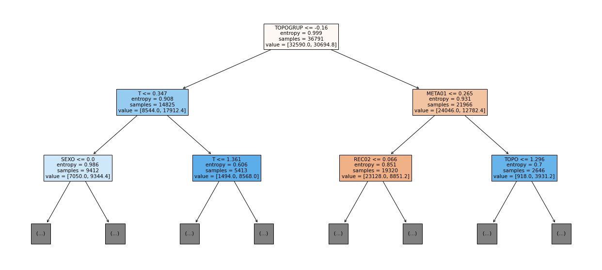
[ ]:
plot_roc_curve(rf_sp_04_07, X_trainSP_04_07, X_testSP_04_07, y_trainSP_04_07, y_testSP_04_07)
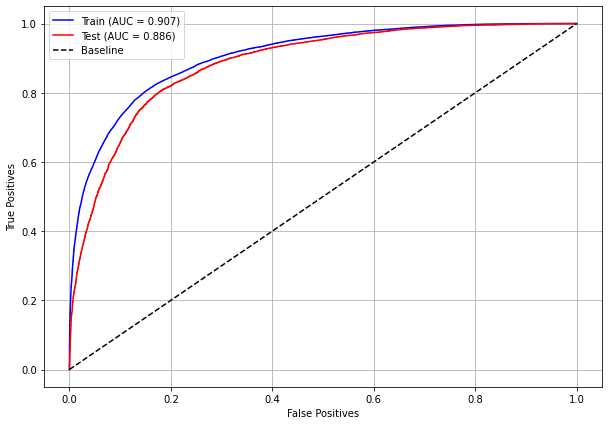
[ ]:
plot_feat_importances(rf_sp_04_07, feat_SP_04_07)
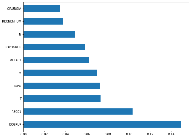
The four most important features in the model were
ECGRUP,REC01,TandTOPO.
[ ]:
plot_shap_values(rf_sp_04_07, X_testSP_04_07, feat_SP_04_07)
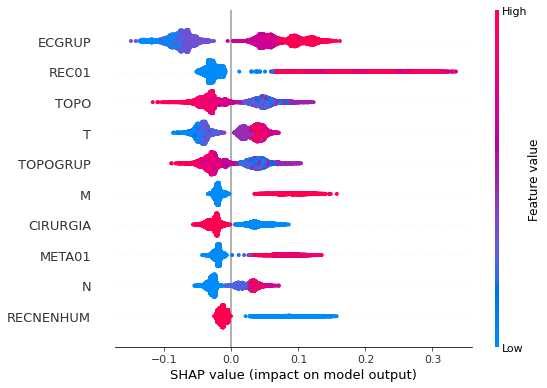
Note that larger values of the ECGRUP column, shown in pink, have more influence for the model’s prediction to be class 1, smaller values have greater weight for the prediction to be class 0. This behavior was expected, because the higher the clinical stage, worse is the stage of cancer.
The other columns shown follow the same logic.
[ ]:
# SP - 2008 to 2011
rf_sp_08_11 = RandomForestClassifier(random_state=seed,
class_weight={0:1, 1:1.475},
criterion='entropy',
max_depth=10)
rf_sp_08_11.fit(X_trainSP_08_11, y_trainSP_08_11)
RandomForestClassifier(class_weight={0: 1, 1: 1.475}, criterion='entropy',
max_depth=10, random_state=10)
[ ]:
display_confusion_matrix(rf_sp_08_11, X_testSP_08_11, y_testSP_08_11)

precision recall f1-score support
0 0.879 0.823 0.850 15705
1 0.749 0.823 0.785 10099
accuracy 0.823 25804
macro avg 0.814 0.823 0.817 25804
weighted avg 0.828 0.823 0.824 25804
The confusion matrix obtained for the Random Forest, with SP data from 2008 to 2011, shows a good performance of the model, with 82% of accuray.
[ ]:
show_tree(rf_sp_08_11, feat_SP_08_11, 2)
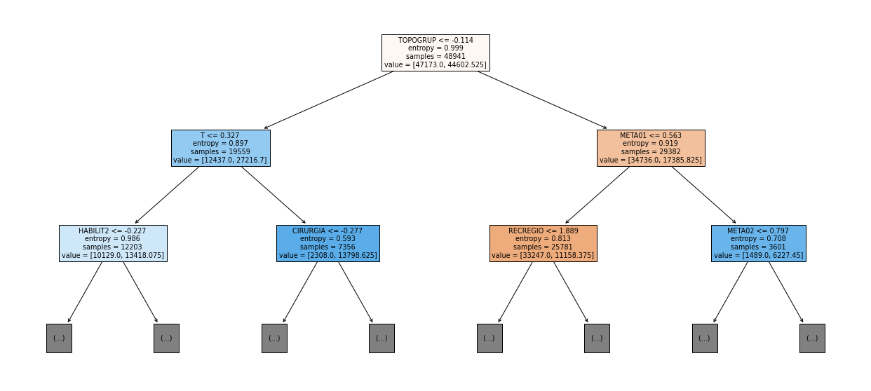
[ ]:
plot_roc_curve(rf_sp_08_11, X_trainSP_08_11, X_testSP_08_11, y_trainSP_08_11, y_testSP_08_11)
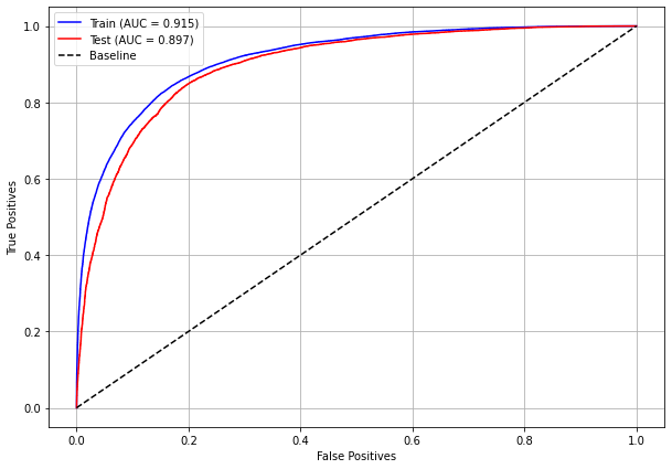
[ ]:
plot_feat_importances(rf_sp_08_11, feat_SP_08_11)
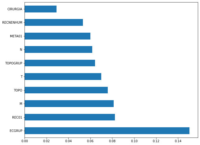
The four most important features in the model were
ECGRUP,REC01,MandTOPO.
[ ]:
plot_shap_values(rf_sp_08_11, X_testSP_08_11, feat_SP_08_11)
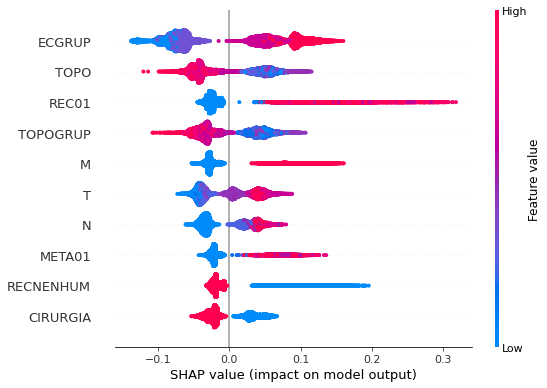
Note that larger values of the ECGRUP column, shown in pink, have more influence for the model’s prediction to be class 1, smaller values have greater weight for the prediction to be class 0. This behavior was expected, because the higher the clinical stage, worse is the stage of cancer.
The other columns shown follow the same logic.
[ ]:
# SP - 2012 to 2015
rf_sp_12_15 = RandomForestClassifier(random_state=seed,
class_weight={0:1, 1:2.05},
criterion='entropy',
max_depth=10)
rf_sp_12_15.fit(X_trainSP_12_15, y_trainSP_12_15)
RandomForestClassifier(class_weight={0: 1, 1: 2.05}, criterion='entropy',
max_depth=10, random_state=10)
[ ]:
display_confusion_matrix(rf_sp_12_15, X_testSP_12_15, y_testSP_12_15)

precision recall f1-score support
0 0.916 0.837 0.874 21800
1 0.706 0.836 0.766 10242
accuracy 0.837 32042
macro avg 0.811 0.836 0.820 32042
weighted avg 0.849 0.837 0.840 32042
The confusion matrix obtained for the Random Forest, with SP data from 2012 to 2015, shows a good performance of the model with 84% of accuracy.
[ ]:
show_tree(rf_sp_12_15, feat_SP_12_15, 2)
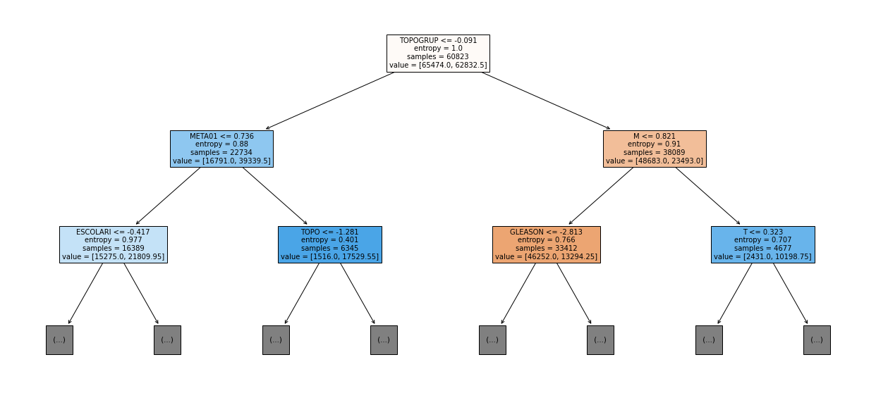
[ ]:
plot_roc_curve(rf_sp_12_15, X_trainSP_12_15, X_testSP_12_15, y_trainSP_12_15, y_testSP_12_15)
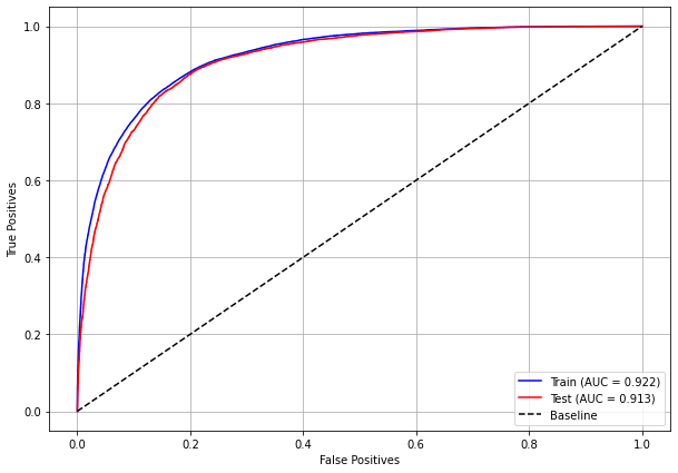
[ ]:
plot_feat_importances(rf_sp_12_15, feat_SP_12_15)
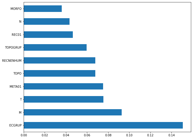
The four most important features in the model were
ECGRUP,M,TandMETA01.
[ ]:
plot_shap_values(rf_sp_12_15, X_testSP_12_15, feat_SP_12_15)
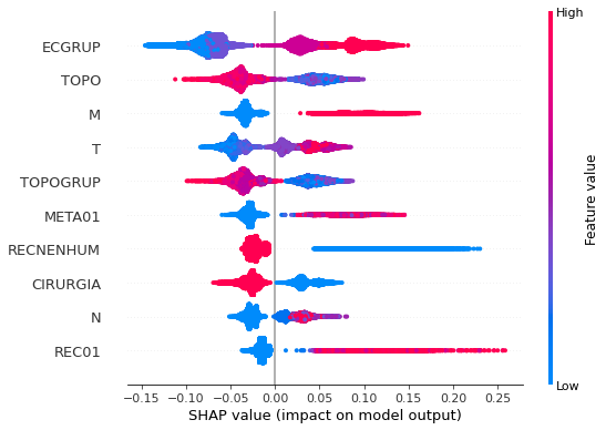
Note that larger values of the ECGRUP column, shown in pink, have more influence for the model’s prediction to be class 1, smaller values have greater weight for the prediction to be class 0. This behavior was expected, because the higher the clinical stage, worse is the stage of cancer.
The other columns shown follow the same logic.
[ ]:
# SP - 2016 to 2021
rf_sp_16_21 = RandomForestClassifier(random_state=seed,
class_weight={0:1, 1:3.015},
criterion='entropy',
max_depth=10)
rf_sp_16_21.fit(X_trainSP_16_21, y_trainSP_16_21)
RandomForestClassifier(class_weight={0: 1, 1: 3.015}, criterion='entropy',
max_depth=10, random_state=10)
[ ]:
display_confusion_matrix(rf_sp_16_21, X_testSP_16_21, y_testSP_16_21)

precision recall f1-score support
0 0.942 0.833 0.884 18758
1 0.607 0.835 0.703 5803
accuracy 0.834 24561
macro avg 0.775 0.834 0.794 24561
weighted avg 0.863 0.834 0.842 24561
The confusion matrix obtained for the Random Forest, with SP data from 2016 to 2021, shows a good performance of the model, with 83% of accuracy.
[ ]:
show_tree(rf_sp_16_21, feat_SP_16_21, 2)
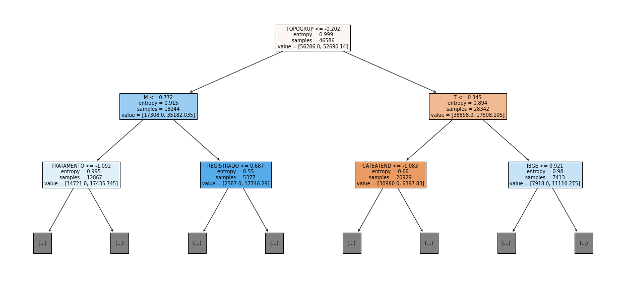
[ ]:
plot_roc_curve(rf_sp_16_21, X_trainSP_16_21, X_testSP_16_21, y_trainSP_16_21, y_testSP_16_21)
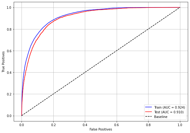
[ ]:
plot_feat_importances(rf_sp_16_21, feat_SP_16_21)
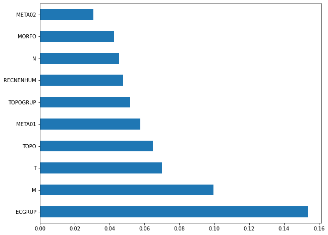
The four most important features in the model were
ECGRUP,M,T, andTOPO.
[ ]:
plot_shap_values(rf_sp_16_21, X_testSP_16_21, feat_SP_16_21)
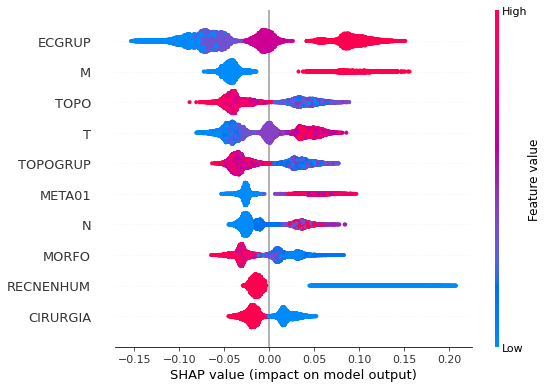
Note that larger values of the ECGRUP column, shown in pink, have more influence for the model’s prediction to be class 1, smaller values have greater weight for the prediction to be class 0. This behavior was expected, because the higher the clinical stage, worse is the stage of cancer.
The other columns shown follow the same logic.
Other states
[ ]:
# Other states - 2000 to 2003
rf_fora_00_03 = RandomForestClassifier(random_state=seed,
class_weight={0:1, 1:1.32},
criterion='entropy',
max_depth=6)
rf_fora_00_03.fit(X_trainOS_00_03, y_trainOS_00_03)
RandomForestClassifier(class_weight={0: 1, 1: 1.32}, criterion='entropy',
max_depth=6, random_state=10)
[ ]:
display_confusion_matrix(rf_fora_00_03, X_testOS_00_03, y_testOS_00_03)

precision recall f1-score support
0 0.781 0.727 0.753 495
1 0.666 0.727 0.695 370
accuracy 0.727 865
macro avg 0.723 0.727 0.724 865
weighted avg 0.732 0.727 0.728 865
The confusion matrix obtained for the Random Forest, with other states data from 2000 to 2003, also shows a good performance of the model, and we have a balanced main diagonal with 73% of accuracy.
[ ]:
show_tree(rf_fora_00_03, feat_OS_00_03, 2)
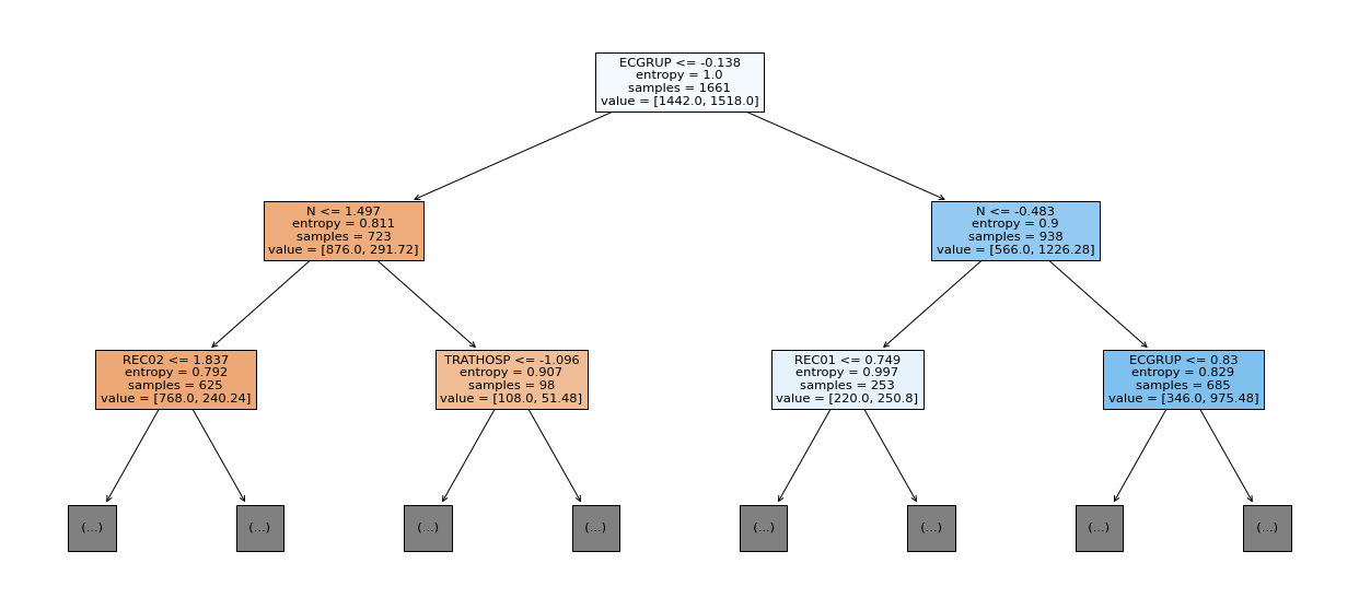
[ ]:
plot_roc_curve(rf_fora_00_03, X_trainOS_00_03, X_testOS_00_03, y_trainOS_00_03, y_testOS_00_03)
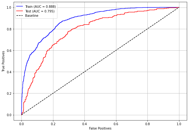
[ ]:
plot_feat_importances(rf_fora_00_03, feat_OS_00_03)
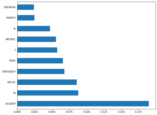
The four most important features in the model were
ECGRUP,M,REC01andTOPOGRUP.
[ ]:
plot_shap_values(rf_fora_00_03, X_testOS_00_03, feat_OS_00_03)
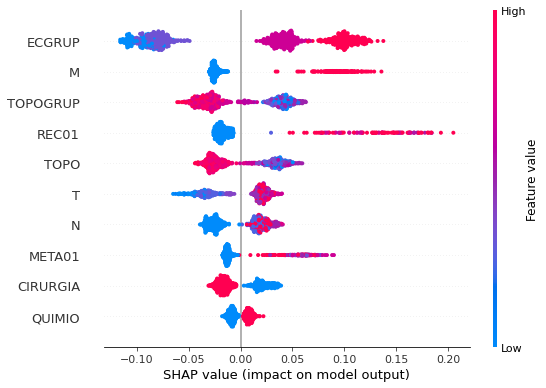
Note that larger values of the ECGRUP column, shown in pink, have more influence for the model’s prediction to be class 1, smaller values have greater weight for the prediction to be class 0. This behavior was expected, because the higher the clinical stage, worse is the stage of cancer.
The other columns shown follow the same logic.
[ ]:
# Other states - 2004 to 2007
rf_fora_04_07 = RandomForestClassifier(random_state=seed,
class_weight={0:1, 1:1.3},
criterion='entropy',
max_depth=6)
rf_fora_04_07.fit(X_trainOS_04_07, y_trainOS_04_07)
RandomForestClassifier(class_weight={0: 1, 1: 1.3}, criterion='entropy',
max_depth=6, random_state=10)
[ ]:
display_confusion_matrix(rf_fora_04_07, X_testOS_04_07, y_testOS_04_07)

precision recall f1-score support
0 0.869 0.822 0.845 724
1 0.764 0.823 0.792 508
accuracy 0.822 1232
macro avg 0.816 0.822 0.818 1232
weighted avg 0.826 0.822 0.823 1232
The confusion matrix obtained for the Random Forest, with other states data from 2004 to 2007, also shows a good performance of the model, with 82% of accuracy.
[ ]:
show_tree(rf_fora_04_07, feat_OS_04_07, 2)
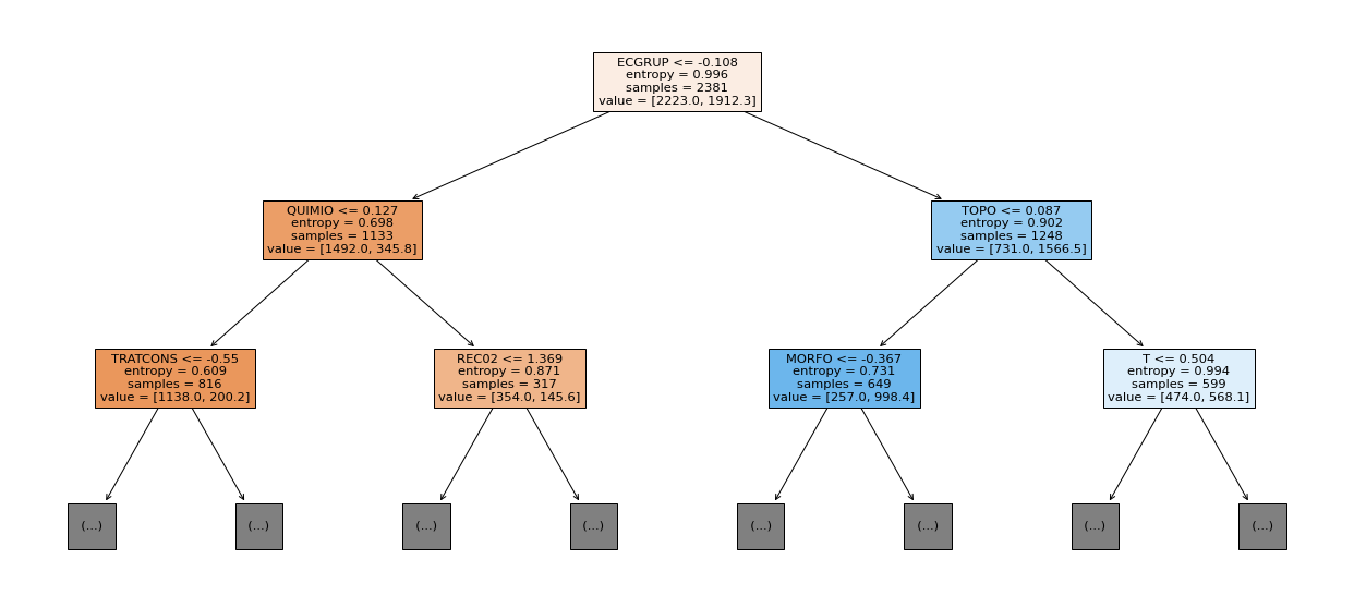
[ ]:
plot_roc_curve(rf_fora_04_07, X_trainOS_04_07, X_testOS_04_07, y_trainOS_04_07, y_testOS_04_07)
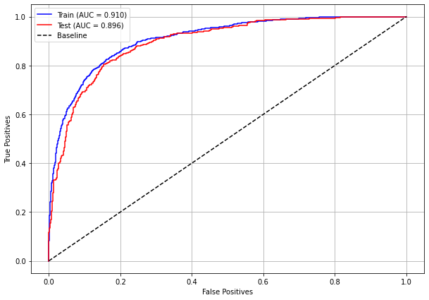
[ ]:
plot_feat_importances(rf_fora_04_07, feat_OS_04_07)
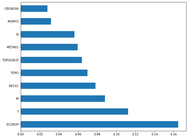
The four most important features in the model were
ECGRUP,T,MandREC01.
[ ]:
plot_shap_values(rf_fora_04_07, X_testOS_04_07, feat_OS_04_07)
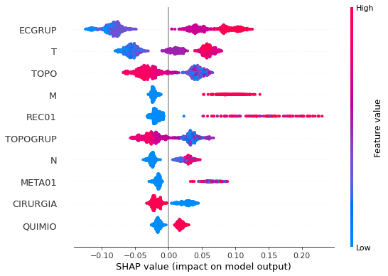
Note that larger values of the ECGRUP column, shown in pink, have more influence for the model’s prediction to be class 1, smaller values have greater weight for the prediction to be class 0. This behavior was expected, because the higher the clinical stage, worse is the stage of cancer.
The other columns shown follow the same logic.
[ ]:
# Other states - 2008 to 2011
rf_fora_08_11 = RandomForestClassifier(random_state=seed,
class_weight={0:1, 1:1.69},
criterion='entropy',
max_depth=6)
rf_fora_08_11.fit(X_trainOS_08_11, y_trainOS_08_11)
RandomForestClassifier(class_weight={0: 1, 1: 1.69}, criterion='entropy',
max_depth=6, random_state=10)
[ ]:
display_confusion_matrix(rf_fora_08_11, X_testOS_08_11, y_testOS_08_11)

precision recall f1-score support
0 0.878 0.805 0.839 962
1 0.702 0.804 0.750 551
accuracy 0.804 1513
macro avg 0.790 0.804 0.795 1513
weighted avg 0.814 0.804 0.807 1513
The confusion matrix obtained for the Random Forest, with other states data from 2008 to 2011, also shows a good performance of the model, presenting 80% of accuracy.
[ ]:
show_tree(rf_fora_08_11, feat_OS_08_11, 2)
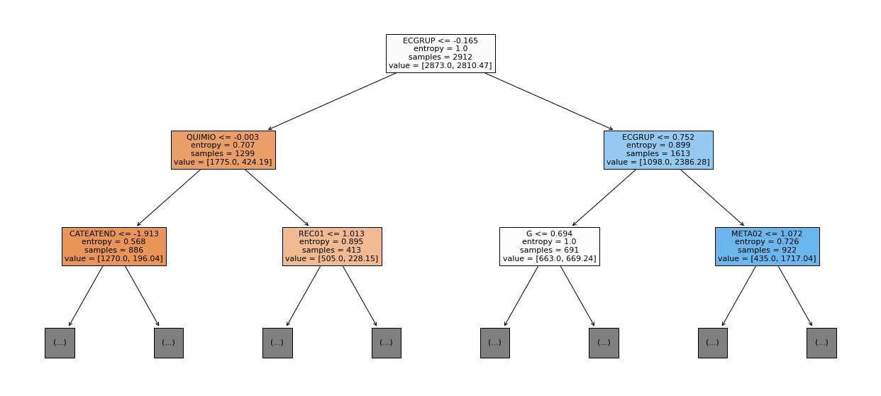
[ ]:
plot_roc_curve(rf_fora_08_11, X_trainOS_08_11, X_testOS_08_11, y_trainOS_08_11, y_testOS_08_11)
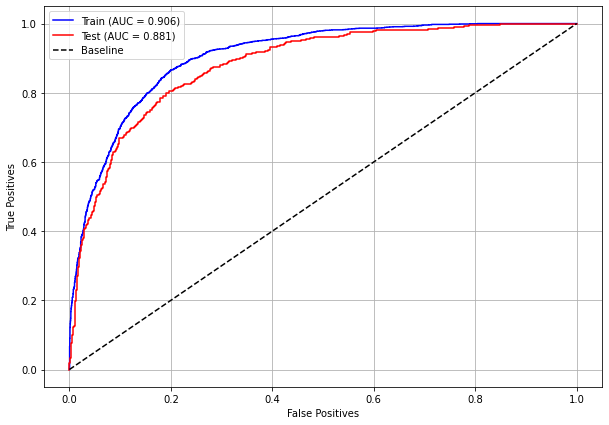
[ ]:
plot_feat_importances(rf_fora_08_11, feat_OS_08_11)
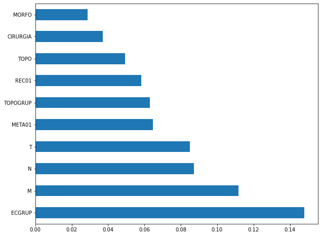
The four most important features in the model were
ECGRUP,M,NandT.
[ ]:
plot_shap_values(rf_fora_08_11, X_testOS_08_11, feat_OS_08_11)
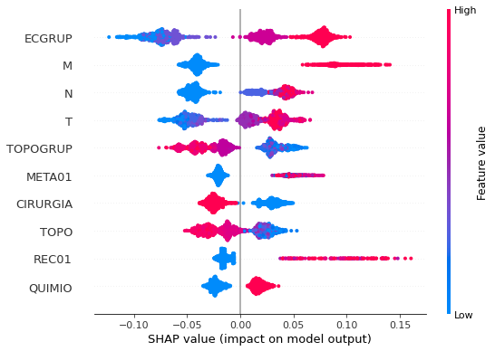
Note that larger values of the ECGRUP column, shown in pink, have more influence for the model’s prediction to be class 1, smaller values have greater weight for the prediction to be class 0. This behavior was expected, because the higher the clinical stage, worse is the stage of cancer.
The other columns shown follow the same logic.
[ ]:
# Other states - 2012 to 2015
rf_fora_12_15 = RandomForestClassifier(random_state=seed,
class_weight={0:1, 1:2.16},
criterion='entropy',
max_depth=6)
rf_fora_12_15.fit(X_trainOS_12_15, y_trainOS_12_15)
RandomForestClassifier(class_weight={0: 1, 1: 2.16}, criterion='entropy',
max_depth=6, random_state=10)
[ ]:
display_confusion_matrix(rf_fora_12_15, X_testOS_12_15, y_testOS_12_15)

precision recall f1-score support
0 0.924 0.833 0.876 1435
1 0.672 0.834 0.744 589
accuracy 0.833 2024
macro avg 0.798 0.833 0.810 2024
weighted avg 0.851 0.833 0.838 2024
The confusion matrix obtained for the Random Forest, with other states data from 2012 to 2015, also shows a good performance of the model, presenting 83% of accuracy.
[ ]:
show_tree(rf_fora_12_15, feat_OS_12_15, 2)
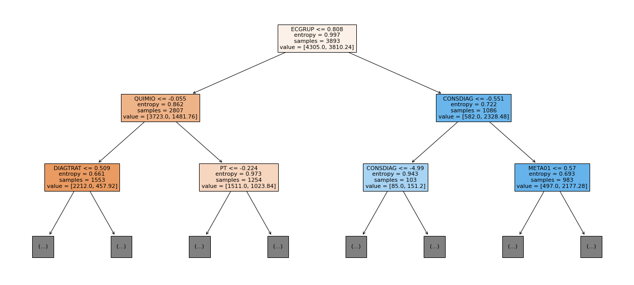
[ ]:
plot_roc_curve(rf_fora_12_15, X_trainOS_12_15, X_testOS_12_15, y_trainOS_12_15, y_testOS_12_15)
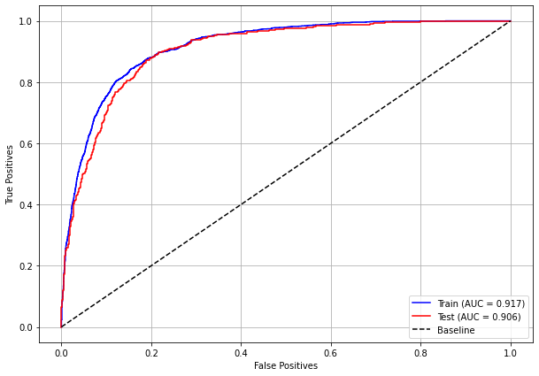
[ ]:
plot_feat_importances(rf_fora_12_15, feat_OS_12_15)
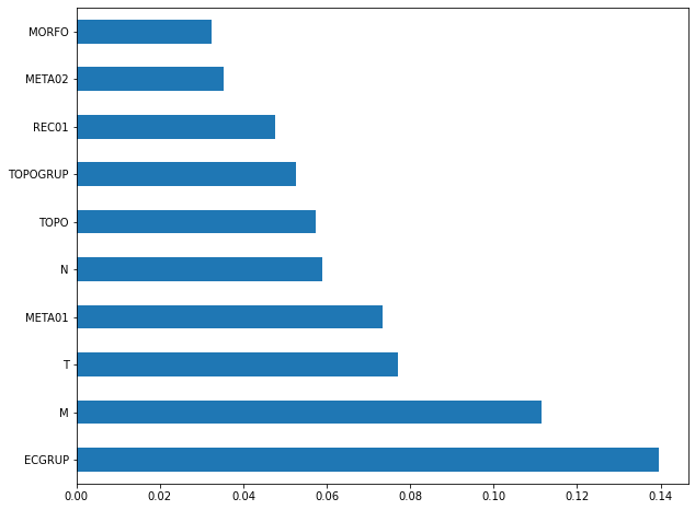
The four most important features in the model were
ECGRUP,M,TandMETA01.
[ ]:
plot_shap_values(rf_fora_12_15, X_testOS_12_15, feat_OS_12_15)
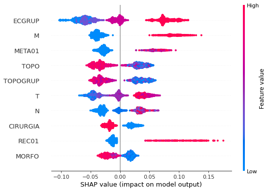
Note that larger values of the ECGRUP column, shown in pink, have more influence for the model’s prediction to be class 1, smaller values have greater weight for the prediction to be class 0. This behavior was expected, because the higher the clinical stage, worse is the stage of cancer.
The other columns shown follow the same logic.
[ ]:
# Other states - 2016 to 2020
rf_fora_16_20 = RandomForestClassifier(random_state=seed,
class_weight={0:1, 1:2.74},
criterion='entropy',
max_depth=7)
rf_fora_16_20.fit(X_trainOS_16_20, y_trainOS_16_20)
RandomForestClassifier(class_weight={0: 1, 1: 2.74}, criterion='entropy',
max_depth=7, random_state=10)
[ ]:
display_confusion_matrix(rf_fora_16_20, X_testOS_16_20, y_testOS_16_20)

precision recall f1-score support
0 0.939 0.830 0.881 1563
1 0.609 0.832 0.703 499
accuracy 0.830 2062
macro avg 0.774 0.831 0.792 2062
weighted avg 0.859 0.830 0.838 2062
The confusion matrix obtained for the Random Forest, with other states data from 2016 to 2020, also shows a good performance of the model, presenting 83% of accuracy.
[ ]:
show_tree(rf_fora_16_20, feat_OS_16_20, 2)
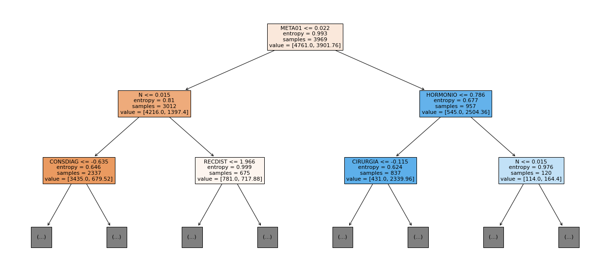
[ ]:
plot_roc_curve(rf_fora_16_20, X_trainOS_16_20, X_testOS_16_20, y_trainOS_16_20, y_testOS_16_20)
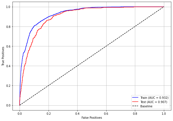
[ ]:
plot_feat_importances(rf_fora_16_20, feat_OS_16_20)
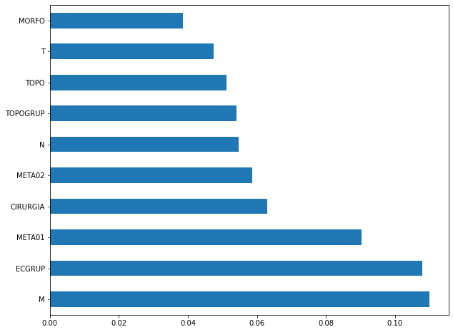
The four most important features in the model were
M,ECGRUP,META01andCIRURGIA.
[ ]:
plot_shap_values(rf_fora_16_20, X_testOS_16_20, feat_OS_16_20)
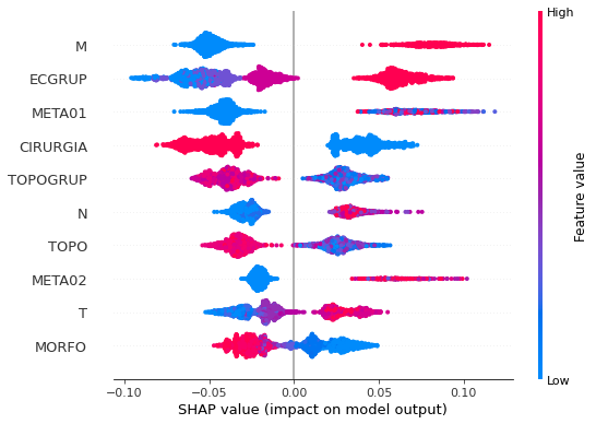
Note that larger values of the M column, shown in pink, have more influence for the model’s prediction to be class 1, smaller values have greater weight for the prediction to be class 0.
The other columns shown follow the same logic.
XGBoost
The training of the XGBoost models follows the same pattern with random_state. The hyperparameter scale_pos_weight was also used in the trainings, in order to obtain a balanced main diagonal in the confusion matrix.
The hyperparameter max_depth was chosen as 10 because the default value for this hyperparameter is 3, a low value for the amount of data we have.
SP
[ ]:
# SP - 2000 to 2003
xgb_sp_00_03 = XGBClassifier(max_depth=8,
random_state=seed,
scale_pos_weight=1.023)
xgb_sp_00_03.fit(X_trainSP_00_03, y_trainSP_00_03)
XGBClassifier(max_depth=8, random_state=10, scale_pos_weight=1.023)
[ ]:
display_confusion_matrix(xgb_sp_00_03, X_testSP_00_03, y_testSP_00_03)
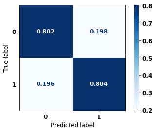
precision recall f1-score support
0 0.815 0.802 0.808 7965
1 0.791 0.804 0.797 7402
accuracy 0.803 15367
macro avg 0.803 0.803 0.803 15367
weighted avg 0.803 0.803 0.803 15367
The confusion matrix obtained for the XGBoost, with SP data from 2000 to 2003, shows a good performance of the model, here with 80% of accuracy.
[ ]:
plot_roc_curve(xgb_sp_00_03, X_trainSP_00_03, X_testSP_00_03, y_trainSP_00_03, y_testSP_00_03)
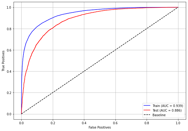
[ ]:
plot_feat_importances(xgb_sp_00_03, feat_SP_00_03)
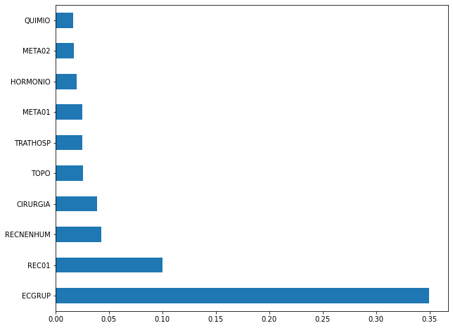
Here we noticed that the most used feature was
ECGRUP, with a lot of advantage over the others. Following we haveREC01,RECNENHUMandCIRURGIA.
[ ]:
plot_shap_values(xgb_sp_00_03, X_testSP_00_03, feat_SP_00_03)
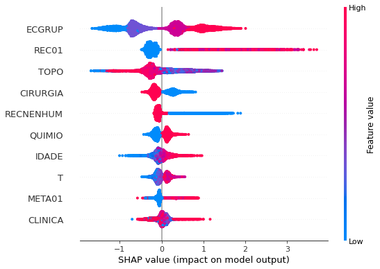
Note that larger values of the ECGRUP column, shown in pink, have more influence for the model’s prediction to be class 1, smaller values have greater weight for the prediction to be class 0. This behavior was expected, because the higher the clinical stage, worse is the stage of cancer.
The other columns shown follow the same logic.
[ ]:
# SP - 2004 to 2007
xgb_sp_04_07 = XGBClassifier(max_depth=8,
random_state=seed,
scale_pos_weight=1.285)
xgb_sp_04_07.fit(X_trainSP_04_07, y_trainSP_04_07)
XGBClassifier(max_depth=8, random_state=10, scale_pos_weight=1.285)
[ ]:
display_confusion_matrix(xgb_sp_04_07, X_testSP_04_07, y_testSP_04_07)

precision recall f1-score support
0 0.859 0.825 0.842 10925
1 0.785 0.826 0.805 8465
accuracy 0.825 19390
macro avg 0.822 0.825 0.823 19390
weighted avg 0.827 0.825 0.826 19390
The confusion matrix obtained for the XGBoost, with SP data from 2004 to 2007, shows a good performance of the model, with 82% of accuracy.
[ ]:
plot_roc_curve(xgb_sp_04_07, X_trainSP_04_07, X_testSP_04_07, y_trainSP_04_07, y_testSP_04_07)

[ ]:
plot_feat_importances(xgb_sp_04_07, feat_SP_04_07)
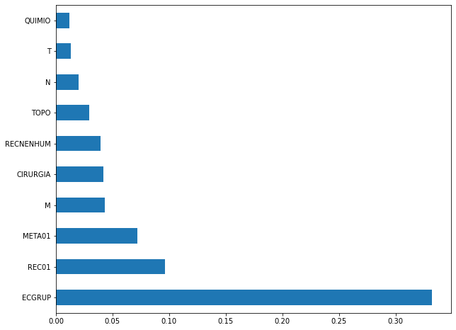
Here we noticed that the most used feature was
ECGRUP, with a good advantage over the others. Following we haveREC01,META01andM.
[ ]:
plot_shap_values(xgb_sp_04_07, X_testSP_04_07, feat_SP_04_07)
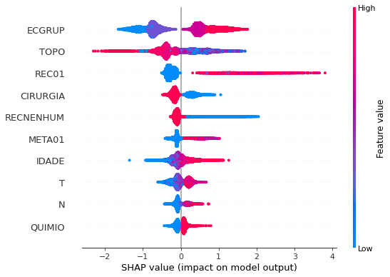
Note that larger values of the ECGRUP column, shown in pink, have more influence for the model’s prediction to be class 1, smaller values have greater weight for the prediction to be class 0. This behavior was expected, because the higher the clinical stage, worse is the stage of cancer.
The other columns shown follow the same logic.
[ ]:
# SP - 2008 to 2011
xgb_sp_08_11 = XGBClassifier(max_depth=8,
scale_pos_weight=1.52,
random_state=seed)
xgb_sp_08_11.fit(X_trainSP_08_11, y_trainSP_08_11)
XGBClassifier(max_depth=8, random_state=10, scale_pos_weight=1.52)
[ ]:
display_confusion_matrix(xgb_sp_08_11, X_testSP_08_11, y_testSP_08_11)
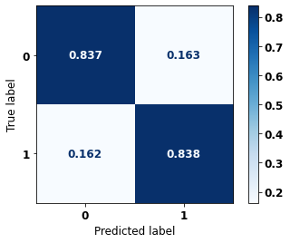
precision recall f1-score support
0 0.889 0.837 0.862 15705
1 0.768 0.838 0.801 10099
accuracy 0.837 25804
macro avg 0.829 0.838 0.832 25804
weighted avg 0.842 0.837 0.839 25804
The confusion matrix obtained for the XGBoost, with SP data from 2008 to 2011, shows a good performance of the model, with 84% of accuracy.
[ ]:
plot_roc_curve(xgb_sp_08_11, X_trainSP_08_11, X_testSP_08_11, y_trainSP_08_11, y_testSP_08_11)
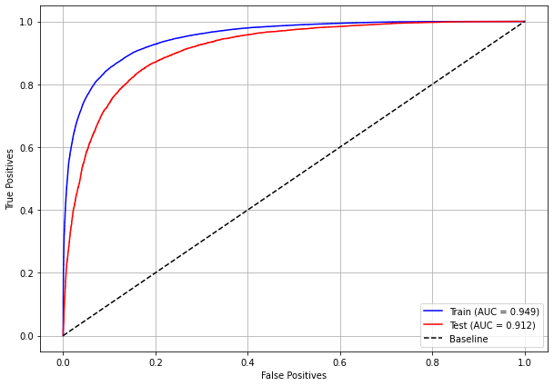
[ ]:
plot_feat_importances(xgb_sp_08_11, feat_SP_08_11)
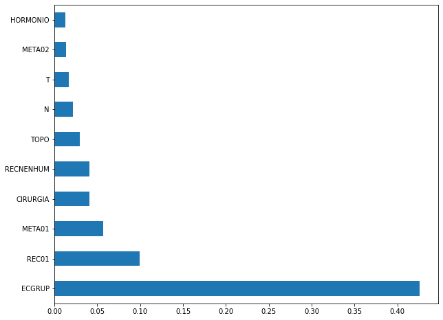
Here we noticed that the most used feature was
ECGRUP, with a good advantage over the others. Following we haveREC01,META01andCIRURGIA.
[ ]:
plot_shap_values(xgb_sp_08_11, X_testSP_08_11, feat_SP_08_11)
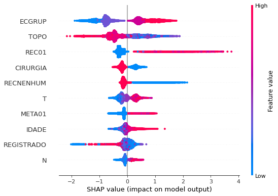
Note that larger values of the ECGRUP column, shown in pink, have more influence for the model’s prediction to be class 1, smaller values have greater weight for the prediction to be class 0. This behavior was expected, because the higher the clinical stage, worse is the stage of cancer.
The other columns shown follow the same logic.
[ ]:
# SP - 2012 to 2015
xgb_sp_12_15 = XGBClassifier(max_depth=8,
random_state=seed,
scale_pos_weight=2.07)
xgb_sp_12_15.fit(X_trainSP_12_15, y_trainSP_12_15)
XGBClassifier(max_depth=8, random_state=10, scale_pos_weight=2.07)
[ ]:
display_confusion_matrix(xgb_sp_12_15, X_testSP_12_15, y_testSP_12_15)

precision recall f1-score support
0 0.924 0.850 0.885 21800
1 0.727 0.851 0.784 10242
accuracy 0.850 32042
macro avg 0.826 0.850 0.835 32042
weighted avg 0.861 0.850 0.853 32042
The confusion matrix obtained for the XGBoost, with SP data from 2012 to 2015, shows a good performance of the model, with 85% of accuracy.
[ ]:
plot_roc_curve(xgb_sp_12_15, X_trainSP_12_15, X_testSP_12_15, y_trainSP_12_15, y_testSP_12_15)

[ ]:
plot_feat_importances(xgb_sp_12_15, feat_SP_12_15)
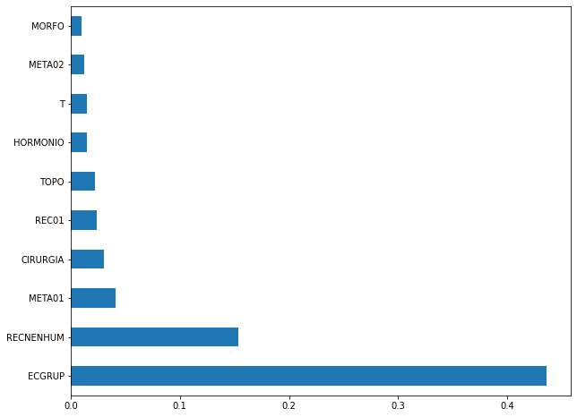
Here we noticed that the most used feature was
ECGRUP, with some advantage. Following we haveRECNENHUM,META01andCIRURGIA.
[ ]:
plot_shap_values(xgb_sp_12_15, X_testSP_12_15, feat_SP_12_15)
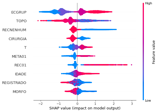
Note that larger values of the ECGRUP column, shown in pink, have more influence for the model’s prediction to be class 1, smaller values have greater weight for the prediction to be class 0. This behavior was expected, because the higher the clinical stage, worse is the stage of cancer.
The other columns shown follow the same logic.
[ ]:
# SP - 2016 to 2021
xgb_sp_16_21 = XGBClassifier(max_depth=8,
random_state=seed,
scale_pos_weight=3.05)
xgb_sp_16_21.fit(X_trainSP_16_21, y_trainSP_16_21)
XGBClassifier(max_depth=8, random_state=10, scale_pos_weight=3.05)
[ ]:
display_confusion_matrix(xgb_sp_16_21, X_testSP_16_21, y_testSP_16_21)

precision recall f1-score support
0 0.949 0.852 0.898 18758
1 0.640 0.852 0.731 5803
accuracy 0.852 24561
macro avg 0.795 0.852 0.815 24561
weighted avg 0.876 0.852 0.859 24561
The confusion matrix obtained for the XGBoost, with SP data from 2016 to 2021, shows a good performance of the model, with 85% of accuracy.
[ ]:
plot_roc_curve(xgb_sp_16_21, X_trainSP_16_21, X_testSP_16_21, y_trainSP_16_21, y_testSP_16_21)

[ ]:
plot_feat_importances(xgb_sp_16_21, feat_SP_16_21)
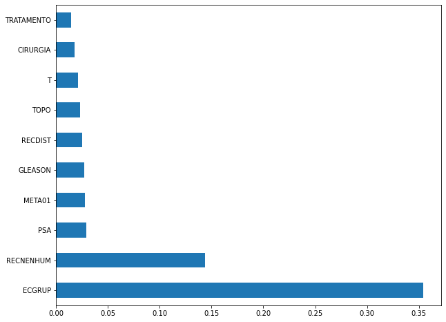
The four most important features were
ECGRUP,RECNENHUM,PSAandMETA01.
[ ]:
plot_shap_values(xgb_sp_16_21, X_testSP_16_21, feat_SP_16_21)
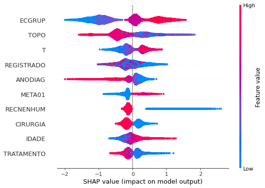
Note that larger values of the ECGRUP column, shown in pink, have more influence for the model’s prediction to be class 1, smaller values have greater weight for the prediction to be class 0. This behavior was expected, because the higher the clinical stage, worse is the stage of cancer.
The other columns shown follow the same logic.
Other states
[ ]:
# Other states - 2000 to 2003
xgb_fora_00_03 = XGBClassifier(max_depth=5,
scale_pos_weight=1.29,
random_state=seed)
xgb_fora_00_03.fit(X_trainOS_00_03, y_trainOS_00_03)
XGBClassifier(max_depth=5, random_state=10, scale_pos_weight=1.29)
[ ]:
display_confusion_matrix(xgb_fora_00_03, X_testOS_00_03, y_testOS_00_03)

precision recall f1-score support
0 0.781 0.729 0.754 495
1 0.667 0.727 0.696 370
accuracy 0.728 865
macro avg 0.724 0.728 0.725 865
weighted avg 0.733 0.728 0.729 865
The confusion matrix obtained for the XGBoost, with other states data from 2000 to 2003, also shows a good performance of the model, with 73% of accuracy.
[ ]:
plot_roc_curve(xgb_fora_00_03, X_trainOS_00_03, X_testOS_00_03, y_trainOS_00_03, y_testOS_00_03)
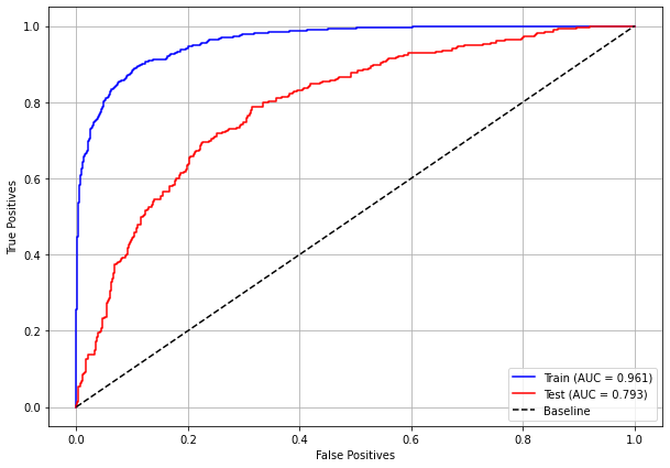
[ ]:
plot_feat_importances(xgb_fora_00_03, feat_OS_00_03)
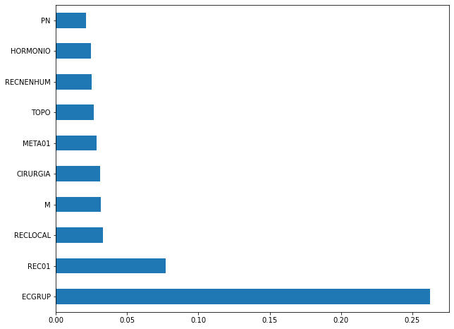
Again we noticed that the most used feature was
ECGRUP, with a good advantage. The following most important features wereREC01,RECLOCALandM.
[ ]:
plot_shap_values(xgb_fora_00_03, X_testOS_00_03, feat_OS_00_03)
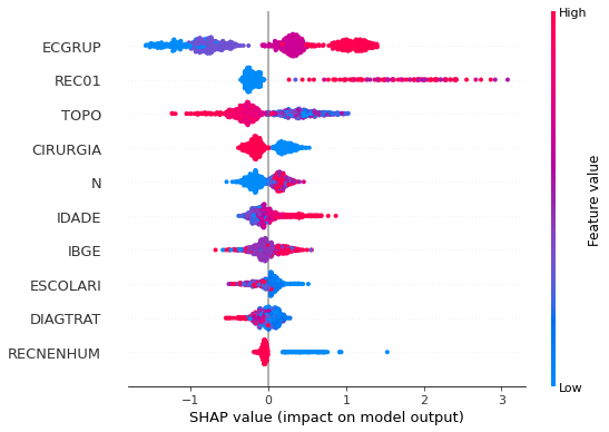
Note that larger values of the ECGRUP column, shown in pink, have more influence for the model’s prediction to be class 1, smaller values have greater weight for the prediction to be class 0. This behavior was expected, because the higher the clinical stage, worse is the stage of cancer.
The other columns shown follow the same logic.
[ ]:
# Other states - 2004 to 2007
xgb_fora_04_07 = XGBClassifier(max_depth=5,
scale_pos_weight=1.5,
random_state=seed)
xgb_fora_04_07.fit(X_trainOS_04_07, y_trainOS_04_07)
XGBClassifier(max_depth=5, random_state=10, scale_pos_weight=1.5)
[ ]:
display_confusion_matrix(xgb_fora_04_07, X_testOS_04_07, y_testOS_04_07)

precision recall f1-score support
0 0.874 0.831 0.852 724
1 0.775 0.829 0.801 508
accuracy 0.830 1232
macro avg 0.825 0.830 0.827 1232
weighted avg 0.833 0.830 0.831 1232
The confusion matrix obtained for the XGBoost, with other states data from 2004 to 2007, also shows a good performance of the model with 83% of accuracy.
[ ]:
plot_roc_curve(xgb_fora_04_07, X_trainOS_04_07, X_testOS_04_07, y_trainOS_04_07, y_testOS_04_07)
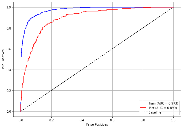
[ ]:
plot_feat_importances(xgb_fora_04_07, feat_OS_04_07)
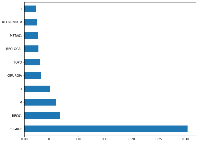
Again we noticed that the most used feature was
ECGRUP, with a good advantage. The following most important features wereREC01,MandT.
[ ]:
plot_shap_values(xgb_fora_04_07, X_testOS_04_07, feat_OS_04_07)
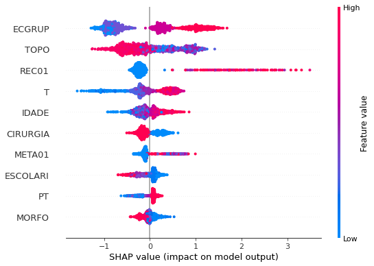
Note that larger values of the ECGRUP column, shown in pink, have more influence for the model’s prediction to be class 1, smaller values have greater weight for the prediction to be class 0. This behavior was expected, because the higher the clinical stage, worse is the stage of cancer.
The other columns shown follow the same logic.
[ ]:
# Other states - 2008 to 2011
xgb_fora_08_11 = XGBClassifier(max_depth=5,
scale_pos_weight=1.87,
random_state=seed)
xgb_fora_08_11.fit(X_trainOS_08_11, y_trainOS_08_11)
XGBClassifier(max_depth=5, random_state=10, scale_pos_weight=1.87)
[ ]:
display_confusion_matrix(xgb_fora_08_11, X_testOS_08_11, y_testOS_08_11)

precision recall f1-score support
0 0.882 0.810 0.844 962
1 0.710 0.811 0.757 551
accuracy 0.810 1513
macro avg 0.796 0.811 0.801 1513
weighted avg 0.819 0.810 0.813 1513
The confusion matrix obtained for the XGBoost, with other states from 2008 to 2011, also shows a good performance of the model with 81% of accuracy.
[ ]:
plot_roc_curve(xgb_fora_08_11, X_trainOS_08_11, X_testOS_08_11, y_trainOS_08_11, y_testOS_08_11)
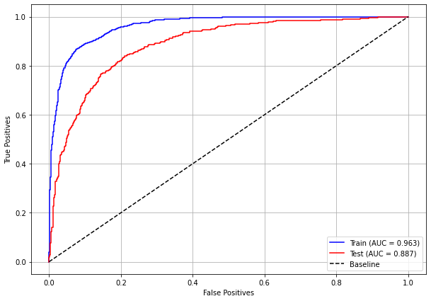
[ ]:
plot_feat_importances(xgb_fora_08_11, feat_OS_08_11)
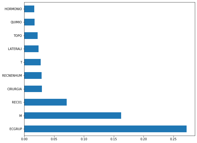
Again we noticed that the most used feature was
ECGRUP, but not with a lot of advantage. The following most important features wereM,REC01andCIRURGIA.
[ ]:
plot_shap_values(xgb_fora_08_11, X_testOS_08_11, feat_OS_08_11)
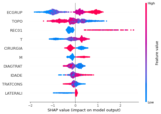
Note that larger values of the ECGRUP column, shown in pink, have more influence for the model’s prediction to be class 1, smaller values have greater weight for the prediction to be class 0. This behavior was expected, because the higher the clinical stage, worse is the stage of cancer.
The other columns shown follow the same logic.
[ ]:
# Other states - 2012 to 2015
xgb_fora_12_15 = XGBClassifier(max_depth=6,
scale_pos_weight=2.57,
random_state=seed)
xgb_fora_12_15.fit(X_trainOS_12_15, y_trainOS_12_15)
XGBClassifier(max_depth=6, random_state=10, scale_pos_weight=2.57)
[ ]:
display_confusion_matrix(xgb_fora_12_15, X_testOS_12_15, y_testOS_12_15)
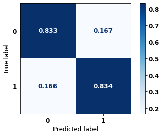
precision recall f1-score support
0 0.924 0.833 0.877 1435
1 0.673 0.834 0.745 589
accuracy 0.833 2024
macro avg 0.798 0.834 0.811 2024
weighted avg 0.851 0.833 0.838 2024
The confusion matrix obtained for the XGBoost, with other states data from 2012 to 2015, also shows a good performance of the model with 83% of accuracy.
[ ]:
plot_roc_curve(xgb_fora_12_15, X_trainOS_12_15, X_testOS_12_15, y_trainOS_12_15, y_testOS_12_15)
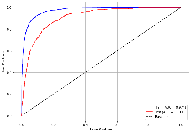
[ ]:
plot_feat_importances(xgb_fora_12_15, feat_OS_12_15)
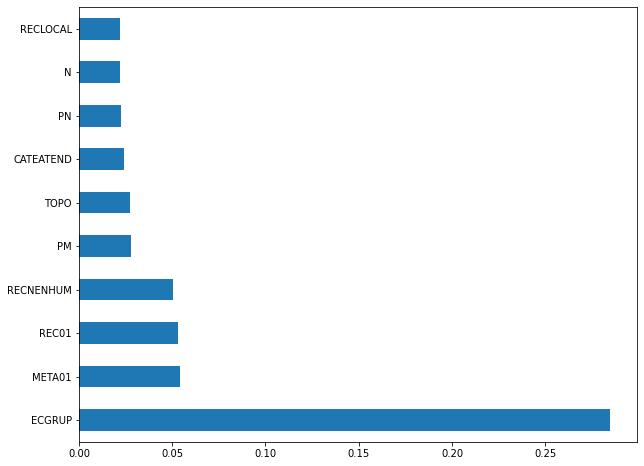
The four most important features were
ECGRUP,META01,REC01andRECNENHUM.
[ ]:
plot_shap_values(xgb_fora_12_15, X_testOS_12_15, feat_OS_12_15)
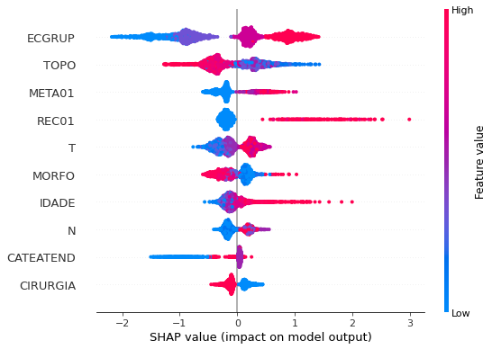
Note that larger values of the ECGRUP column, shown in pink, have more influence for the model’s prediction to be class 1, smaller values have greater weight for the prediction to be class 0. This behavior was expected, because the higher the clinical stage, worse is the stage of cancer.
The other columns shown follow the same logic.
[ ]:
# Other states - 2016 to 2020
xgb_fora_16_20 = XGBClassifier(max_depth=6,
scale_pos_weight=3.38,
random_state=seed)
xgb_fora_16_20.fit(X_trainOS_16_20, y_trainOS_16_20)
XGBClassifier(max_depth=6, random_state=10, scale_pos_weight=3.38)
[ ]:
display_confusion_matrix(xgb_fora_16_20, X_testOS_16_20, y_testOS_16_20)

precision recall f1-score support
0 0.943 0.843 0.891 1563
1 0.632 0.842 0.722 499
accuracy 0.843 2062
macro avg 0.788 0.842 0.806 2062
weighted avg 0.868 0.843 0.850 2062
The confusion matrix obtained for the XGBoost, with other states from 2016 to 2020, shows the best performance comparing with the other models, with 84% of accuracy.
[ ]:
plot_roc_curve(xgb_fora_16_20, X_trainOS_16_20, X_testOS_16_20, y_trainOS_16_20, y_testOS_16_20)
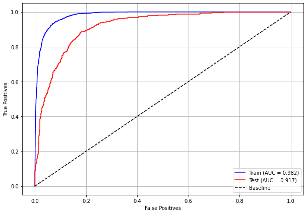
[ ]:
plot_feat_importances(xgb_fora_16_20, feat_OS_16_20)
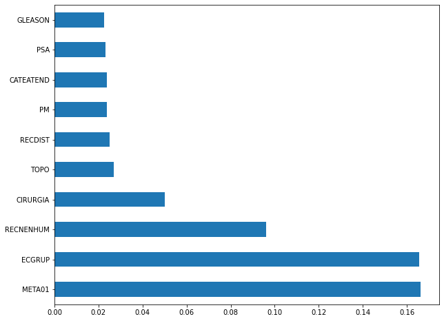
The four most important features were
META01,ECGRUP,RECNENHUMandCIRURGIA.
[ ]:
plot_shap_values(xgb_fora_16_20, X_testOS_16_20, feat_OS_16_20)
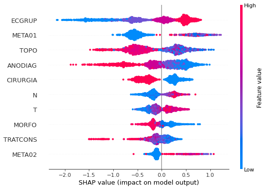
Note that larger values of the ECGRUP column, shown in pink, have more influence for the model’s prediction to be class 1, smaller values have greater weight for the prediction to be class 0. This behavior was expected, because the higher the clinical stage, worse is the stage of cancer.
The other columns shown follow the same logic.
Testing models with data from other years
We will use test data from the following years in the trained models for each set of years grouped together.
Random Forest SP for years 2000 to 2003
[ ]:
display_confusion_matrix(rf_sp_00_03, X_testSP_04_07, y_testSP_04_07)

precision recall f1-score support
0 0.847 0.799 0.822 10925
1 0.758 0.814 0.785 8465
accuracy 0.806 19390
macro avg 0.803 0.806 0.804 19390
weighted avg 0.808 0.806 0.806 19390
[ ]:
display_confusion_matrix(rf_sp_00_03, X_testSP_08_11, y_testSP_08_11)
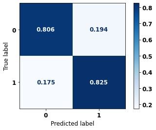
precision recall f1-score support
0 0.877 0.806 0.840 15705
1 0.732 0.825 0.776 10099
accuracy 0.813 25804
macro avg 0.805 0.815 0.808 25804
weighted avg 0.821 0.813 0.815 25804
[ ]:
display_confusion_matrix(rf_sp_00_03, X_testSP_12_15, y_testSP_12_15)

precision recall f1-score support
0 0.919 0.803 0.857 21800
1 0.670 0.850 0.749 10242
accuracy 0.818 32042
macro avg 0.794 0.826 0.803 32042
weighted avg 0.839 0.818 0.823 32042
[ ]:
display_confusion_matrix(rf_sp_00_03, X_testSP_16_21, y_testSP_16_21)
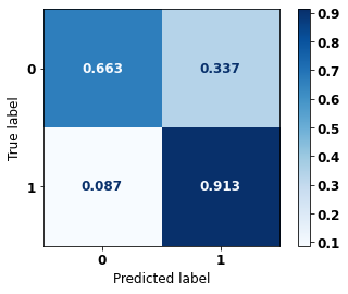
precision recall f1-score support
0 0.961 0.663 0.785 18758
1 0.456 0.913 0.608 5803
accuracy 0.722 24561
macro avg 0.708 0.788 0.696 24561
weighted avg 0.842 0.722 0.743 24561
XGBoost SP for years 2000 to 2003
[ ]:
display_confusion_matrix(xgb_sp_00_03, X_testSP_04_07, y_testSP_04_07)

precision recall f1-score support
0 0.832 0.828 0.830 10925
1 0.780 0.784 0.782 8465
accuracy 0.809 19390
macro avg 0.806 0.806 0.806 19390
weighted avg 0.809 0.809 0.809 19390
[ ]:
display_confusion_matrix(xgb_sp_00_03, X_testSP_08_11, y_testSP_08_11)

precision recall f1-score support
0 0.860 0.837 0.848 15705
1 0.757 0.788 0.772 10099
accuracy 0.818 25804
macro avg 0.808 0.812 0.810 25804
weighted avg 0.819 0.818 0.818 25804
[ ]:
display_confusion_matrix(xgb_sp_00_03, X_testSP_12_15, y_testSP_12_15)
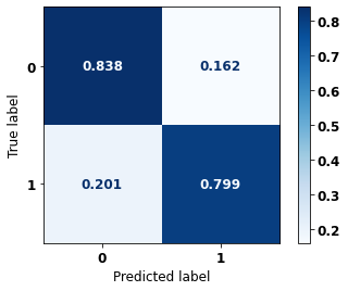
precision recall f1-score support
0 0.899 0.838 0.868 21800
1 0.699 0.799 0.746 10242
accuracy 0.826 32042
macro avg 0.799 0.819 0.807 32042
weighted avg 0.835 0.826 0.829 32042
[ ]:
display_confusion_matrix(xgb_sp_00_03, X_testSP_16_21, y_testSP_16_21)
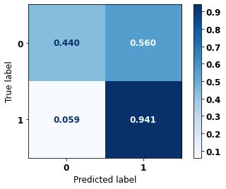
precision recall f1-score support
0 0.960 0.440 0.603 18758
1 0.342 0.941 0.502 5803
accuracy 0.558 24561
macro avg 0.651 0.690 0.553 24561
weighted avg 0.814 0.558 0.579 24561
Random Forest SP for years 2004 to 2007
[ ]:
display_confusion_matrix(rf_sp_04_07, X_testSP_08_11, y_testSP_08_11)

precision recall f1-score support
0 0.879 0.813 0.845 15705
1 0.740 0.826 0.781 10099
accuracy 0.818 25804
macro avg 0.809 0.820 0.813 25804
weighted avg 0.825 0.818 0.820 25804
[ ]:
display_confusion_matrix(rf_sp_04_07, X_testSP_12_15, y_testSP_12_15)

precision recall f1-score support
0 0.919 0.805 0.858 21800
1 0.671 0.850 0.750 10242
accuracy 0.819 32042
macro avg 0.795 0.827 0.804 32042
weighted avg 0.840 0.819 0.824 32042
[ ]:
display_confusion_matrix(rf_sp_04_07, X_testSP_16_21, y_testSP_16_21)

precision recall f1-score support
0 0.960 0.680 0.796 18758
1 0.468 0.908 0.617 5803
accuracy 0.734 24561
macro avg 0.714 0.794 0.707 24561
weighted avg 0.843 0.734 0.754 24561
XGBoost SP for years 2004 to 2007
[ ]:
display_confusion_matrix(xgb_sp_04_07, X_testSP_08_11, y_testSP_08_11)

precision recall f1-score support
0 0.880 0.825 0.851 15705
1 0.751 0.824 0.786 10099
accuracy 0.825 25804
macro avg 0.815 0.825 0.819 25804
weighted avg 0.829 0.825 0.826 25804
[ ]:
display_confusion_matrix(xgb_sp_04_07, X_testSP_12_15, y_testSP_12_15)

precision recall f1-score support
0 0.905 0.745 0.817 21800
1 0.605 0.834 0.702 10242
accuracy 0.773 32042
macro avg 0.755 0.789 0.759 32042
weighted avg 0.809 0.773 0.780 32042
[ ]:
display_confusion_matrix(xgb_sp_04_07, X_testSP_16_21, y_testSP_16_21)
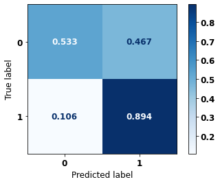
precision recall f1-score support
0 0.942 0.533 0.681 18758
1 0.372 0.894 0.525 5803
accuracy 0.618 24561
macro avg 0.657 0.713 0.603 24561
weighted avg 0.807 0.618 0.644 24561
Random Forest SP for years 2008 to 2011
[ ]:
display_confusion_matrix(rf_sp_08_11, X_testSP_12_15, y_testSP_12_15)

precision recall f1-score support
0 0.923 0.808 0.862 21800
1 0.677 0.857 0.757 10242
accuracy 0.824 32042
macro avg 0.800 0.833 0.809 32042
weighted avg 0.845 0.824 0.828 32042
[ ]:
display_confusion_matrix(rf_sp_08_11, X_testSP_16_21, y_testSP_16_21)
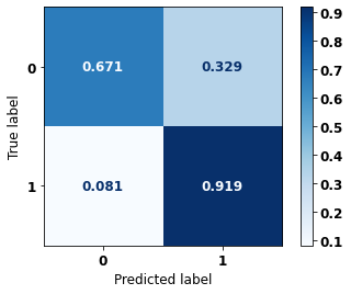
precision recall f1-score support
0 0.964 0.671 0.791 18758
1 0.464 0.919 0.617 5803
accuracy 0.730 24561
macro avg 0.714 0.795 0.704 24561
weighted avg 0.846 0.730 0.750 24561
XGBoost SP for years 2008 to 2011
[ ]:
display_confusion_matrix(xgb_sp_08_11, X_testSP_12_15, y_testSP_12_15)

precision recall f1-score support
0 0.911 0.791 0.847 21800
1 0.652 0.836 0.733 10242
accuracy 0.805 32042
macro avg 0.782 0.813 0.790 32042
weighted avg 0.828 0.805 0.810 32042
[ ]:
display_confusion_matrix(xgb_sp_08_11, X_testSP_16_21, y_testSP_16_21)
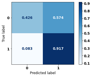
precision recall f1-score support
0 0.943 0.426 0.587 18758
1 0.331 0.917 0.486 5803
accuracy 0.542 24561
macro avg 0.637 0.671 0.536 24561
weighted avg 0.799 0.542 0.563 24561
Random Forest SP for years 2012 to 2015
[ ]:
display_confusion_matrix(rf_sp_12_15, X_testSP_16_21, y_testSP_16_21)

precision recall f1-score support
0 0.948 0.777 0.854 18758
1 0.544 0.862 0.667 5803
accuracy 0.797 24561
macro avg 0.746 0.819 0.760 24561
weighted avg 0.852 0.797 0.810 24561
XGBoost SP for years 2012 to 2015
[ ]:
display_confusion_matrix(xgb_sp_12_15, X_testSP_16_21, y_testSP_16_21)

precision recall f1-score support
0 0.948 0.793 0.864 18758
1 0.563 0.859 0.680 5803
accuracy 0.809 24561
macro avg 0.755 0.826 0.772 24561
weighted avg 0.857 0.809 0.820 24561
Random Forest Other states for years 2000 to 2003
[ ]:
display_confusion_matrix(rf_fora_00_03, X_testOS_04_07, y_testOS_04_07)

precision recall f1-score support
0 0.852 0.819 0.835 724
1 0.756 0.797 0.776 508
accuracy 0.810 1232
macro avg 0.804 0.808 0.806 1232
weighted avg 0.812 0.810 0.811 1232
[ ]:
display_confusion_matrix(rf_fora_00_03, X_testOS_08_11, y_testOS_08_11)

precision recall f1-score support
0 0.882 0.771 0.823 962
1 0.673 0.820 0.739 551
accuracy 0.789 1513
macro avg 0.777 0.796 0.781 1513
weighted avg 0.806 0.789 0.793 1513
[ ]:
display_confusion_matrix(rf_fora_00_03, X_testOS_12_15, y_testOS_12_15)
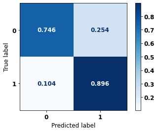
precision recall f1-score support
0 0.946 0.746 0.834 1435
1 0.591 0.896 0.713 589
accuracy 0.790 2024
macro avg 0.769 0.821 0.773 2024
weighted avg 0.843 0.790 0.799 2024
[ ]:
display_confusion_matrix(rf_fora_00_03, X_testOS_16_20, y_testOS_16_20)
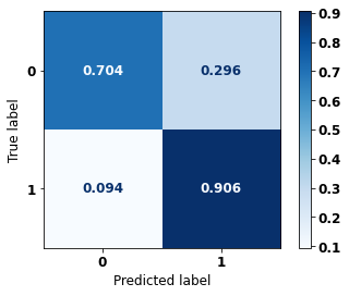
precision recall f1-score support
0 0.959 0.704 0.812 1563
1 0.495 0.906 0.640 499
accuracy 0.753 2062
macro avg 0.727 0.805 0.726 2062
weighted avg 0.847 0.753 0.771 2062
XGBoost Other states for years 2000 to 2003
[ ]:
display_confusion_matrix(xgb_fora_00_03, X_testOS_04_07, y_testOS_04_07)

precision recall f1-score support
0 0.860 0.840 0.850 724
1 0.779 0.805 0.792 508
accuracy 0.825 1232
macro avg 0.820 0.822 0.821 1232
weighted avg 0.827 0.825 0.826 1232
[ ]:
display_confusion_matrix(xgb_fora_00_03, X_testOS_08_11, y_testOS_08_11)

precision recall f1-score support
0 0.881 0.786 0.831 962
1 0.685 0.815 0.745 551
accuracy 0.796 1513
macro avg 0.783 0.800 0.788 1513
weighted avg 0.810 0.796 0.799 1513
[ ]:
display_confusion_matrix(xgb_fora_00_03, X_testOS_12_15, y_testOS_12_15)
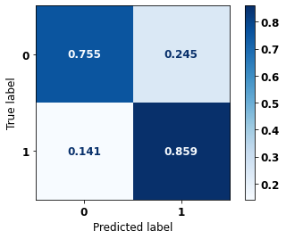
precision recall f1-score support
0 0.929 0.755 0.833 1435
1 0.590 0.859 0.700 589
accuracy 0.786 2024
macro avg 0.760 0.807 0.767 2024
weighted avg 0.830 0.786 0.794 2024
[ ]:
display_confusion_matrix(xgb_fora_00_03, X_testOS_16_20, y_testOS_16_20)
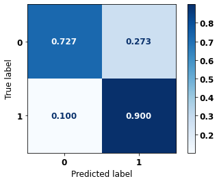
precision recall f1-score support
0 0.958 0.727 0.826 1563
1 0.513 0.900 0.653 499
accuracy 0.769 2062
macro avg 0.735 0.813 0.740 2062
weighted avg 0.850 0.769 0.785 2062
Random Forest Other states for years 2004 to 2007
[ ]:
display_confusion_matrix(rf_fora_04_07, X_testOS_08_11, y_testOS_08_11)

precision recall f1-score support
0 0.880 0.785 0.830 962
1 0.684 0.813 0.743 551
accuracy 0.795 1513
macro avg 0.782 0.799 0.786 1513
weighted avg 0.809 0.795 0.798 1513
[ ]:
display_confusion_matrix(rf_fora_04_07, X_testOS_12_15, y_testOS_12_15)
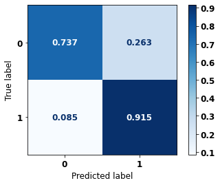
precision recall f1-score support
0 0.955 0.737 0.832 1435
1 0.588 0.915 0.716 589
accuracy 0.789 2024
macro avg 0.772 0.826 0.774 2024
weighted avg 0.848 0.789 0.798 2024
[ ]:
display_confusion_matrix(rf_fora_04_07, X_testOS_16_20, y_testOS_16_20)

precision recall f1-score support
0 0.967 0.695 0.809 1563
1 0.492 0.926 0.643 499
accuracy 0.751 2062
macro avg 0.730 0.810 0.726 2062
weighted avg 0.852 0.751 0.768 2062
XGBoost Other states for years 2004 to 2007
[ ]:
display_confusion_matrix(xgb_fora_04_07, X_testOS_08_11, y_testOS_08_11)

precision recall f1-score support
0 0.880 0.810 0.844 962
1 0.709 0.808 0.755 551
accuracy 0.809 1513
macro avg 0.794 0.809 0.799 1513
weighted avg 0.818 0.809 0.811 1513
[ ]:
display_confusion_matrix(xgb_fora_04_07, X_testOS_12_15, y_testOS_12_15)

precision recall f1-score support
0 0.948 0.753 0.839 1435
1 0.599 0.900 0.719 589
accuracy 0.795 2024
macro avg 0.774 0.826 0.779 2024
weighted avg 0.847 0.795 0.804 2024
[ ]:
display_confusion_matrix(xgb_fora_04_07, X_testOS_16_20, y_testOS_16_20)

precision recall f1-score support
0 0.969 0.731 0.833 1563
1 0.524 0.928 0.670 499
accuracy 0.778 2062
macro avg 0.747 0.829 0.751 2062
weighted avg 0.862 0.778 0.794 2062
Random Forest Other states for years 2008 to 2011
[ ]:
display_confusion_matrix(rf_fora_08_11, X_testOS_12_15, y_testOS_12_15)

precision recall f1-score support
0 0.938 0.771 0.847 1435
1 0.611 0.876 0.720 589
accuracy 0.802 2024
macro avg 0.775 0.824 0.783 2024
weighted avg 0.843 0.802 0.810 2024
[ ]:
display_confusion_matrix(rf_fora_08_11, X_testOS_16_20, y_testOS_16_20)
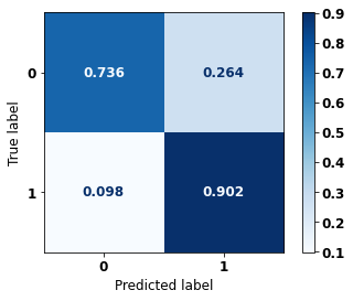
precision recall f1-score support
0 0.959 0.736 0.833 1563
1 0.522 0.902 0.661 499
accuracy 0.776 2062
macro avg 0.741 0.819 0.747 2062
weighted avg 0.853 0.776 0.792 2062
XGBoost Other states for years 2008 to 2011
[ ]:
display_confusion_matrix(xgb_fora_08_11, X_testOS_12_15, y_testOS_12_15)

precision recall f1-score support
0 0.931 0.792 0.856 1435
1 0.628 0.857 0.725 589
accuracy 0.811 2024
macro avg 0.780 0.825 0.790 2024
weighted avg 0.843 0.811 0.818 2024
[ ]:
display_confusion_matrix(xgb_fora_08_11, X_testOS_16_20, y_testOS_16_20)
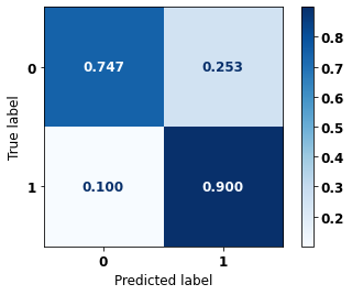
precision recall f1-score support
0 0.959 0.747 0.840 1563
1 0.531 0.900 0.668 499
accuracy 0.784 2062
macro avg 0.745 0.823 0.754 2062
weighted avg 0.855 0.784 0.798 2062
Random Forest Other states for years 2012 to 2015
[ ]:
display_confusion_matrix(rf_fora_12_15, X_testOS_16_20, y_testOS_16_20)

precision recall f1-score support
0 0.950 0.784 0.859 1563
1 0.563 0.870 0.683 499
accuracy 0.805 2062
macro avg 0.756 0.827 0.771 2062
weighted avg 0.856 0.805 0.817 2062
XGBoost Other states for years 2012 to 2015
[ ]:
display_confusion_matrix(xgb_fora_12_15, X_testOS_16_20, y_testOS_16_20)

precision recall f1-score support
0 0.940 0.798 0.863 1563
1 0.570 0.840 0.679 499
accuracy 0.808 2062
macro avg 0.755 0.819 0.771 2062
weighted avg 0.850 0.808 0.818 2062