Introduction
In this section, two machine learning models will be used to classify the vivo_ano1 column, Random Forest and XGBoost, for both datasets, São Paulo and other states.
The label is 1 if the patient is alive after one year of treatment and 0 if not.
The first approach is using the “raw data”, the second is without the EC column, the third one is without EC and HORMONIO, the fourth is using the grouped years and without the column EC and the fifth is also with the years gruped and without EC and HORMONIO.
The years will be grouped as follows: 2000 to 2003, 2004 to 2007, 2008 to 2011, 2012 to 2015 and 2016 until the end. So we will have 5 datasets for SP and another 5 for other states.
Reading the data from SP and other states.
We can see that we still have some missing values in both datasets, but the columns DTRECIDIVA, delta_t4, delta_t5 and delta_t6 will not be used in this approach.
[ ]:
df_SP = read_csv('/content/drive/MyDrive/Trabalho/Cancer/Datasets/geral_sp_labels.csv')
df_fora = read_csv('/content/drive/MyDrive/Trabalho/Cancer/Datasets/geral_fora_sp_labels.csv')
(506037, 77)
(32891, 77)
Here we have the correlations between the label and the other columns, the columns with higher correlations will not be used as features of the models, because they may have been used to create the label, such as the ULTINFO column, or they can be used as label for other machine learning models.
[ ]:
# SP
corr_matrix = df_SP.corr()
abs(corr_matrix['vivo_ano1']).sort_values(ascending = False).head(20)
vivo_ano1       1.000000
vivo_ano3       0.550659
ULTIDIAG        0.516977
ULTICONS        0.511464
ULTITRAT        0.506234
vivo_ano5       0.379191
obito_cancer    0.334877
obito_geral     0.288888
HORMONIO        0.213111
MORFO           0.211231
CIRURGIA        0.200385
RECNENHUM       0.143184
ULTINFO         0.135111
DIAGTRAT        0.109031
CLINICA         0.107280
RECLOCAL        0.098045
TRATCONS        0.078914
RADIO           0.078885
RECDIST         0.068599
SEXO            0.067825
Name: vivo_ano1, dtype: float64
[ ]:
# Other states
corr_matrix = df_fora.corr()
abs(corr_matrix['vivo_ano1']).sort_values(ascending = False).head(20)
vivo_ano1       1.000000
vivo_ano3       0.547481
ULTIDIAG        0.534214
ULTICONS        0.525986
ULTITRAT        0.521397
vivo_ano5       0.365313
obito_cancer    0.313149
obito_geral     0.281608
CIRURGIA        0.225414
HORMONIO        0.188568
MORFO           0.187409
RECNENHUM       0.144844
DIAGTRAT        0.143071
ULTINFO         0.125962
ANODIAG         0.112732
TRATCONS        0.102913
RECDIST         0.099343
RECLOCAL        0.092728
DIAGPREV        0.092233
RADIO           0.081094
Name: vivo_ano1, dtype: float64
Here we have the number of examples for each category of the label, it is clear that there is an imbalance, similar to the previous classification.
[ ]:
df_SP.vivo_ano1.value_counts()
1    382541
0    123496
Name: vivo_ano1, dtype: int64
[ ]:
df_fora.vivo_ano1.value_counts()
1    24709
0     8182
Name: vivo_ano1, dtype: int64
Years of diagnosis present in the data.
[ ]:
np.sort(df_SP.ANODIAG.unique())
array([2000, 2001, 2002, 2003, 2004, 2005, 2006, 2007, 2008, 2009, 2010,
       2011, 2012, 2013, 2014, 2015, 2016, 2017, 2018, 2019, 2020, 2021])
[ ]:
np.sort(df_fora.ANODIAG.unique())
array([2000, 2001, 2002, 2003, 2004, 2005, 2006, 2007, 2008, 2009, 2010,
       2011, 2012, 2013, 2014, 2015, 2016, 2017, 2018, 2019, 2020])
Before dividing the datasets, it is necessary to select only the patients who have been followed up for at least one year.
[ ]:
# SP
df_SP_ano1 = df_SP[~((df_SP.obito_geral == 0) & (df_SP.vivo_ano1 == 0))]
df_SP_ano1.shape
(469704, 77)
[ ]:
# Other States
df_fora_ano1 = df_fora[~((df_fora.obito_geral == 0) & (df_fora.vivo_ano1 == 0))]
df_fora_ano1.shape
(29771, 77)
First approach
Approach with “raw data”.
Preprocessing
Now we are going to divide the data into training and testing, and then do the preprocessing in both datasets to perform the training of the models and their evaluation.
First, it is necessary to define the columns that will be used as features and the label. We will not use some columns of the datasets: UFRESID, because we already have the division between SP and other states in the two datasets.
It was chosen to keep the column IDADE, so we will not use the FAIXAETAR. Finally, the other columns contained in the list list_drop are possible labels, so they will not be used as features for machine learning models.
[ ]:
list_drop = ['UFRESID', 'FAIXAETAR', 'ULTICONS', 'ULTIDIAG', 'ULTITRAT',
             'obito_geral', 'obito_cancer', 'vivo_ano3', 'vivo_ano5', 'ULTINFO']

# 'RECNENHUM', 'RECLOCAL', 'RECREGIO', 'REC01', 'REC02', 'REC03', 'RECDIST'

lb = 'vivo_ano1'
A function was created to perform the preprocessing, preprocessing, that uses the other functions created, get_train_test (divides the dataset into train and test sets), train_preprocessing (do the preprocessing of the train set) and test_preprocessing (do the preprocessing of the test set).
To see the complete function go to the functions section.
SP
[ ]:
X_train_SP, X_test_SP, y_train_SP, y_test_SP, feat_cols_SP = preprocessing(df_SP_ano1, list_drop, lb,
                                                                           random_state=seed,
                                                                           balance_data=False,
                                                                           encoder_type='LabelEncoder',
                                                                           norm_name='StandardScaler')
X_train = (352278, 66), X_test = (117426, 66)
y_train = (352278,), y_test = (117426,)
Other states
[ ]:
X_train_OS, X_test_OS, y_train_OS, y_test_OS, feat_cols_OS = preprocessing(df_fora_ano1, list_drop, lb,
                                                                           random_state=seed,
                                                                           balance_data=False,
                                                                           encoder_type='LabelEncoder',
                                                                           norm_name='StandardScaler')
X_train = (22328, 66), X_test = (7443, 66)
y_train = (22328,), y_test = (7443,)
Training machine learning models
After dividing the data into training and testing, using the encoder and normalizing, the data is ready to be used by the machine learning models.
Random Forest
The first model that will be tested is the Random Forest, for this test the parameter random_state will be used, to obtain the same training values of the model every time it is runned.
The hyperparameter class_weight was also used, because the model has difficulty learning the class with fewer examples, so using this parameter this class will have a higher weight in the training of the model.
[ ]:
# SP
rf_sp = RandomForestClassifier(class_weight={0:4.26, 1:1},
                               random_state=seed,
                               criterion='entropy',
                               max_depth=10)

rf_sp.fit(X_train_SP, y_train_SP)
RandomForestClassifier(class_weight={0: 4.26, 1: 1}, criterion='entropy',
                       max_depth=10, random_state=10)
[ ]:
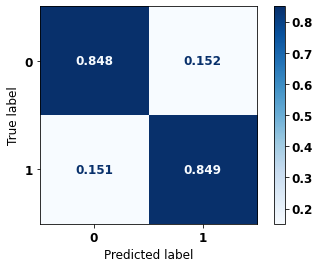
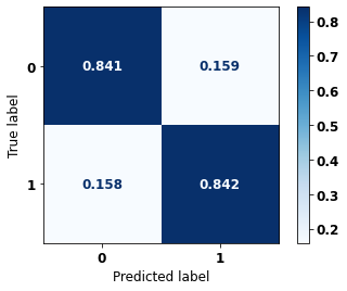
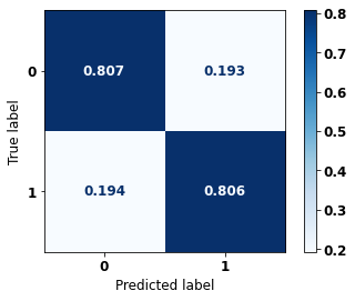
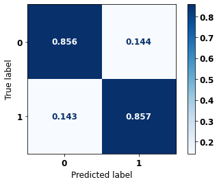
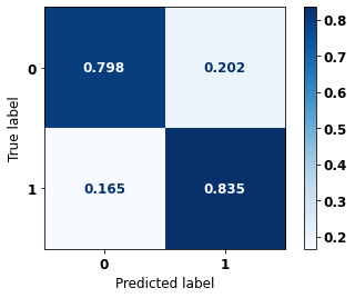
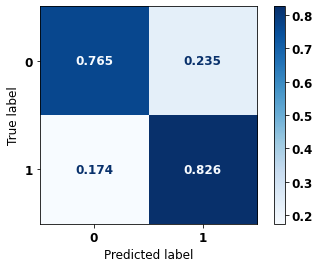
display_confusion_matrix(rf_sp, X_test_SP, y_test_SP)

              precision    recall  f1-score   support

           0      0.514     0.822     0.632     21791
           1      0.953     0.823     0.883     95635

    accuracy                          0.822    117426
   macro avg      0.733     0.822     0.758    117426
weighted avg      0.871     0.822     0.836    117426
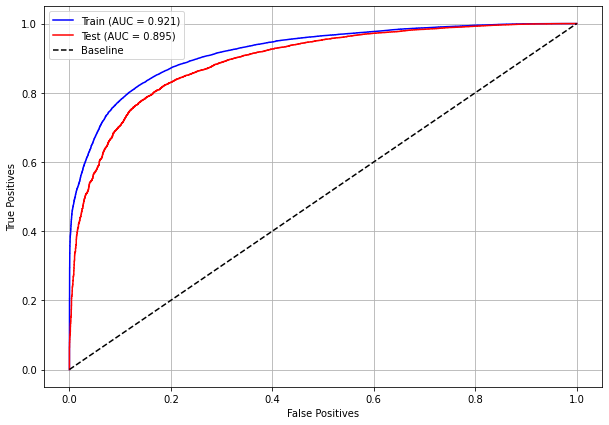
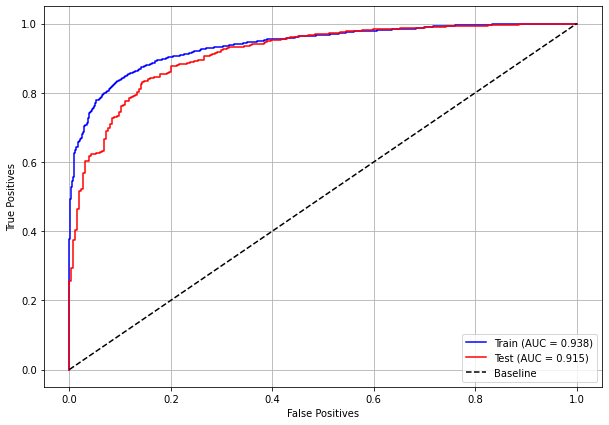
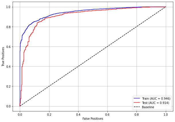
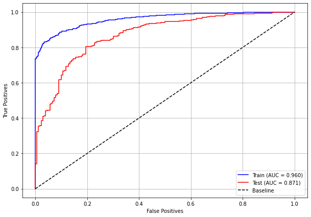
The confusion matrix obtained for the Random Forest, with SP data, shows a good performance of the model, with 82% of accuracy.
[ ]:
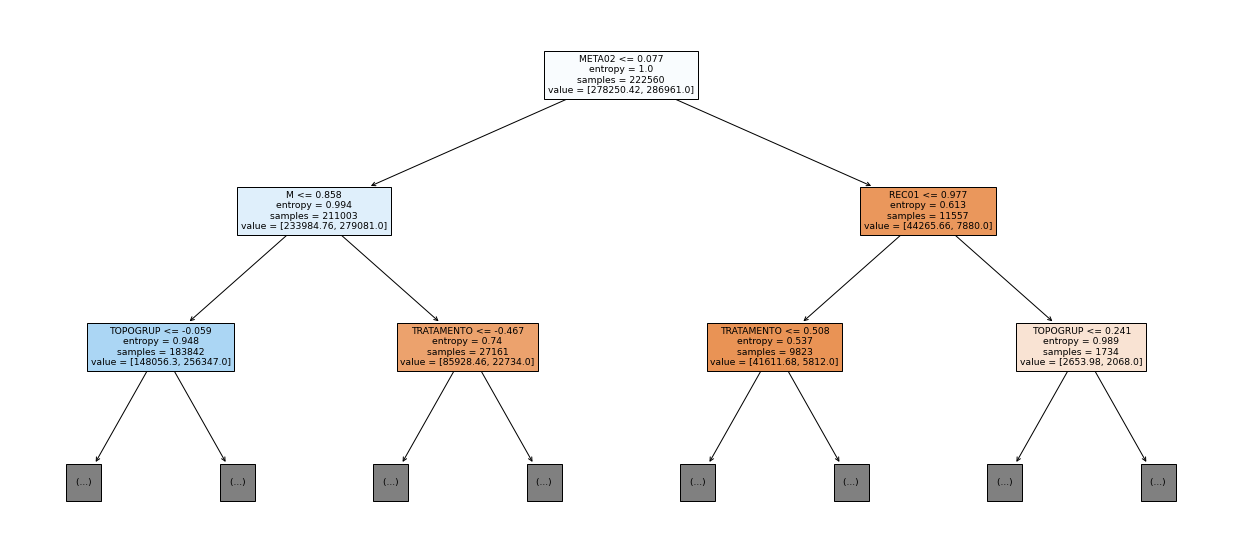
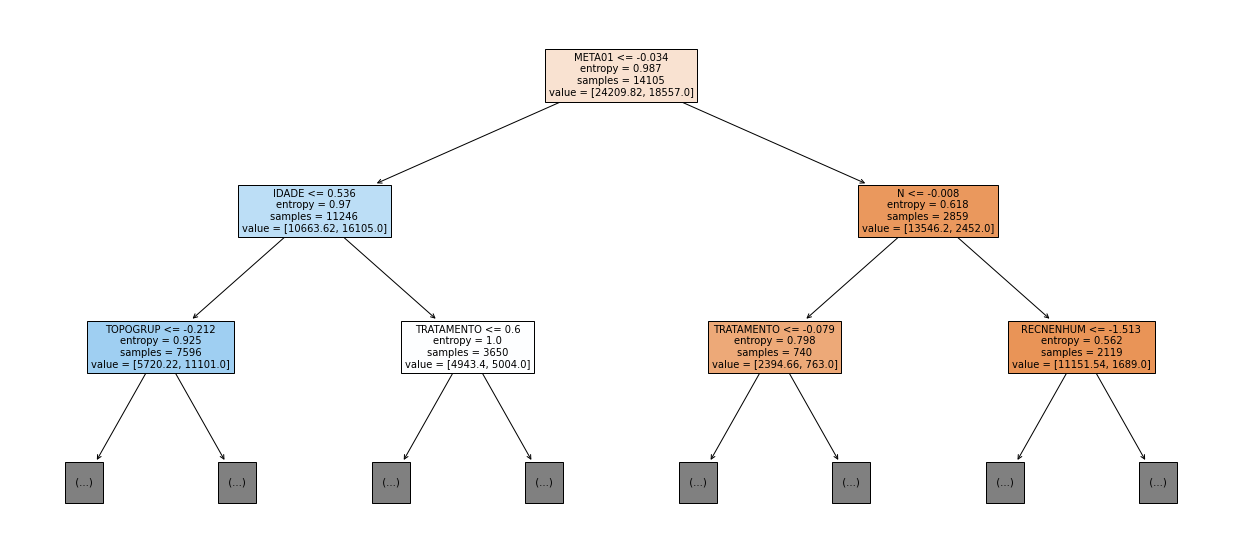
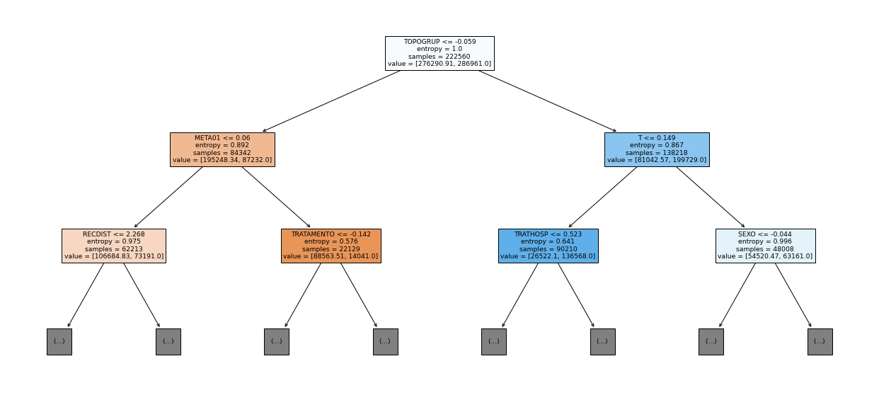
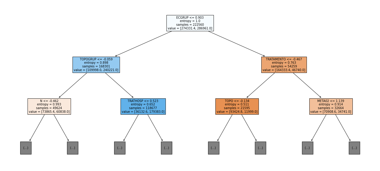
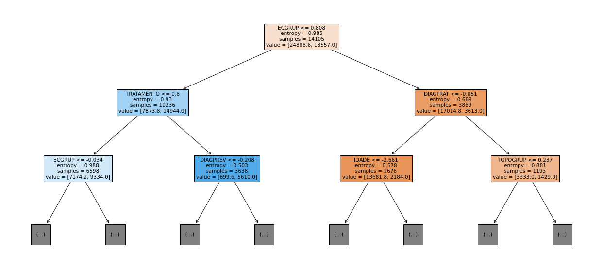
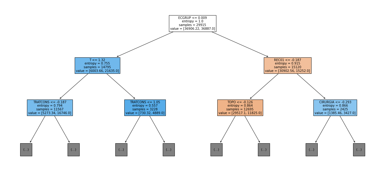
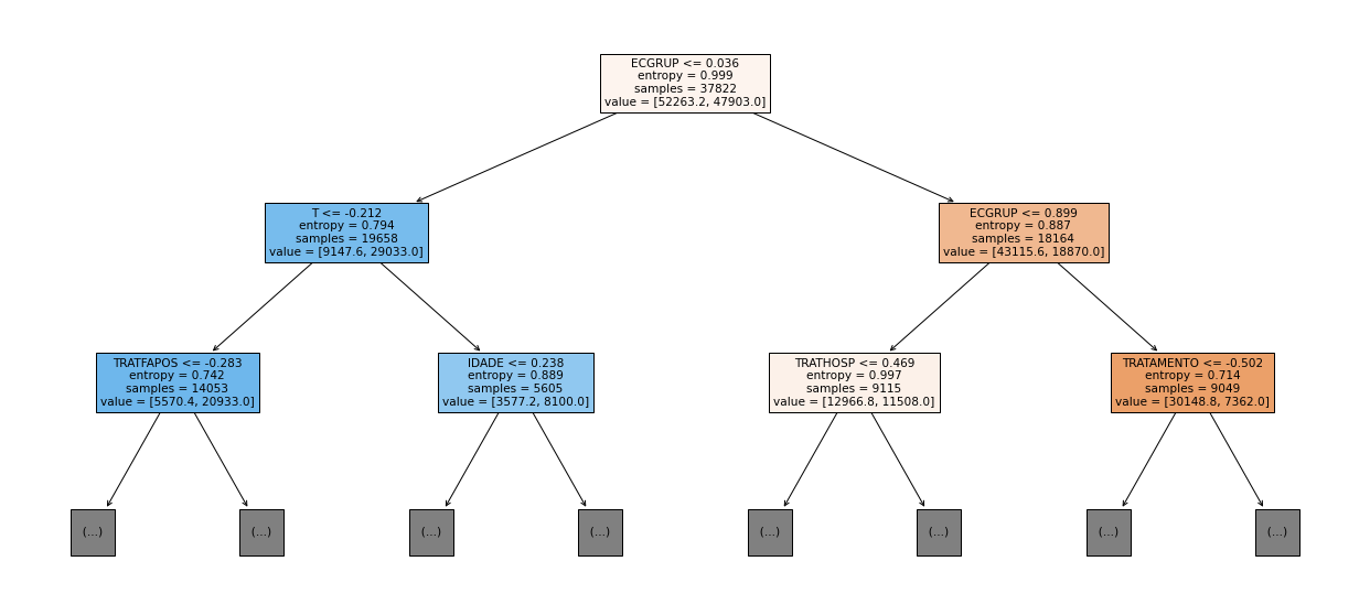
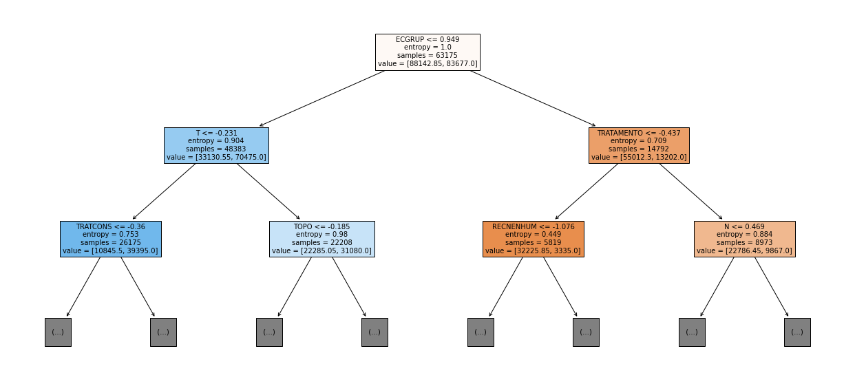
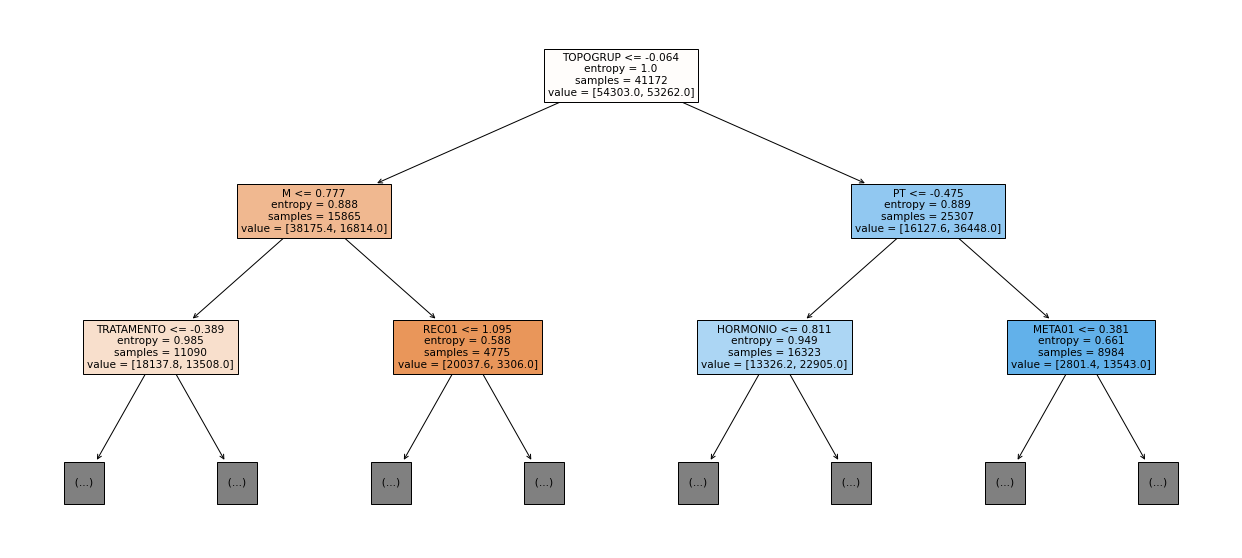
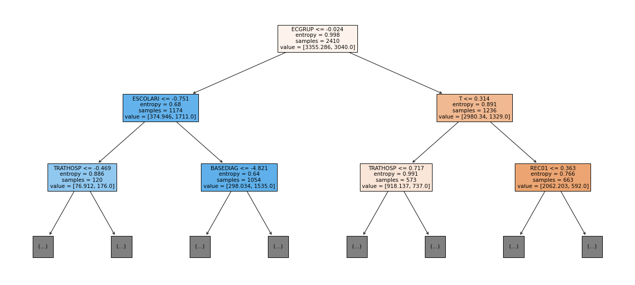
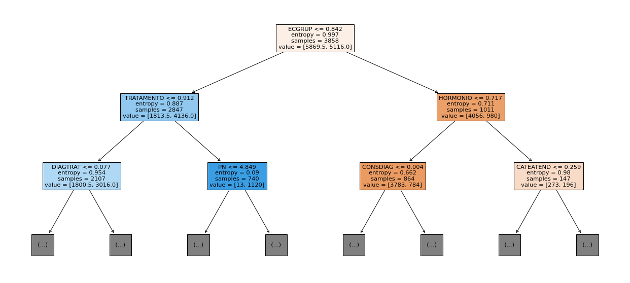
show_tree(rf_sp, feat_cols_SP, 2)
[ ]:
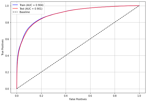
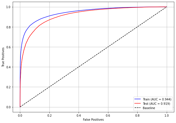
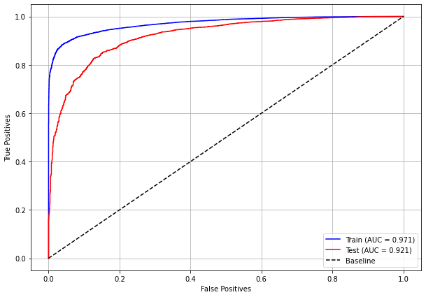
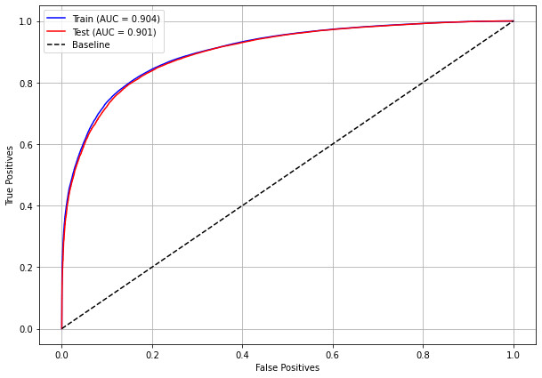
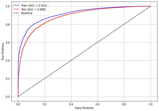
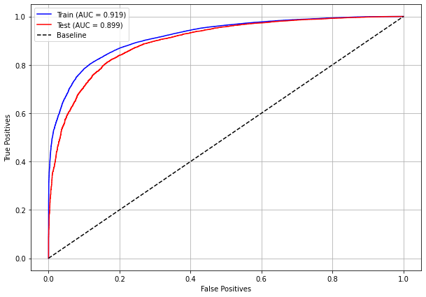
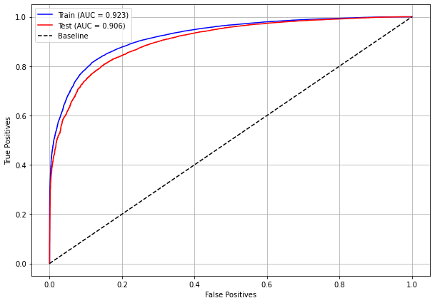
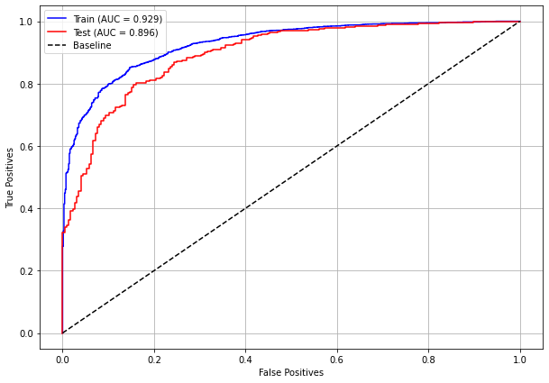
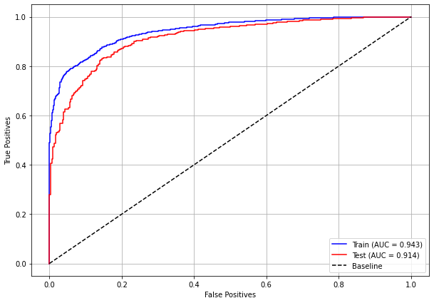
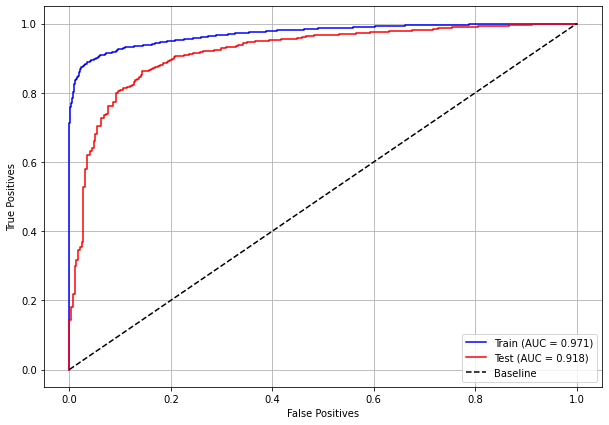
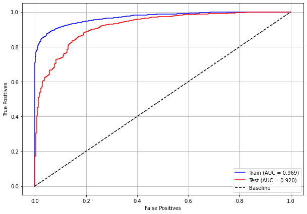
plot_roc_curve(rf_sp, X_train_SP, X_test_SP, y_train_SP, y_test_SP)
[ ]:
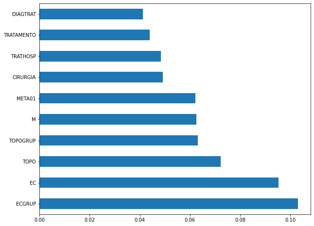
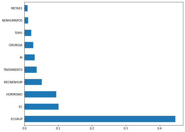
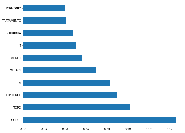
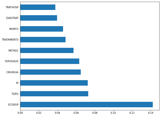
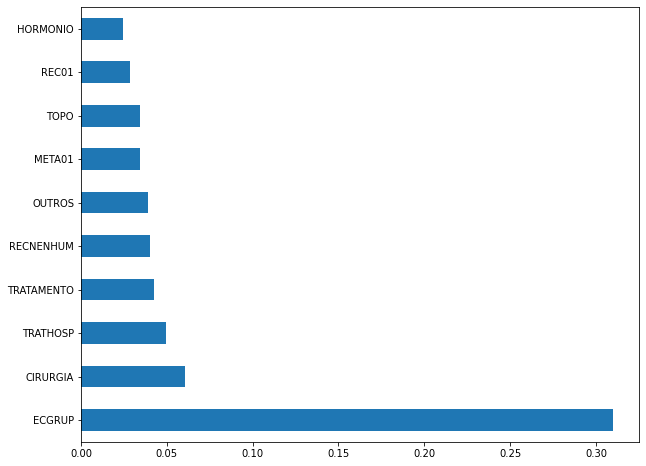
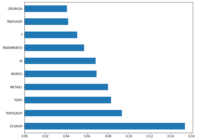
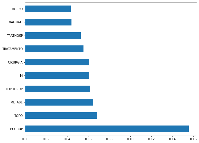
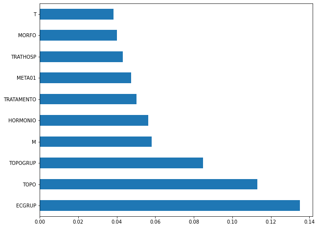
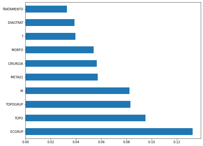
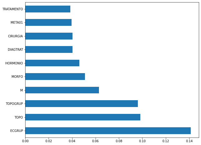
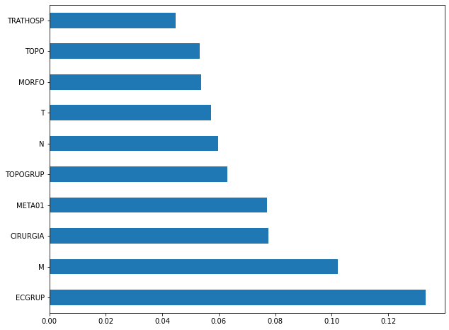
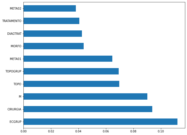
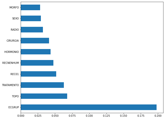
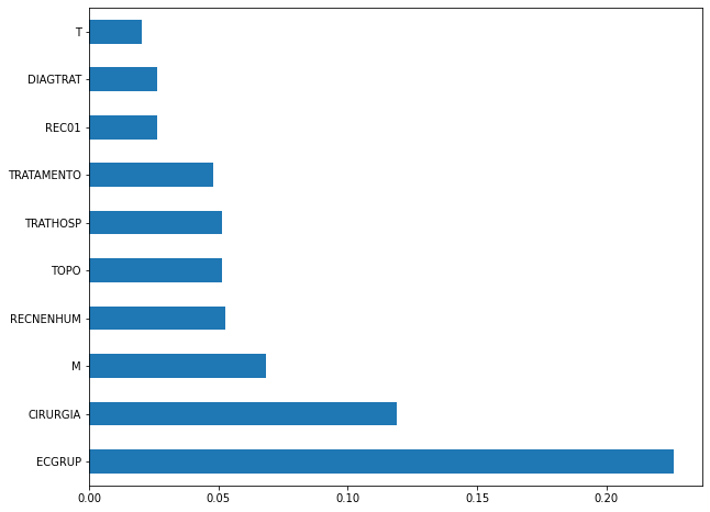
plot_feat_importances(rf_sp, feat_cols_SP)
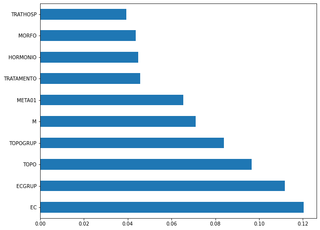
The four most important features in the model were
EC,ECGRUP,TOPOandTOPOGRUP.
[ ]:
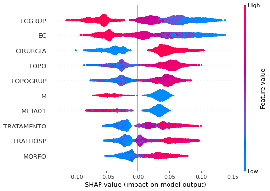
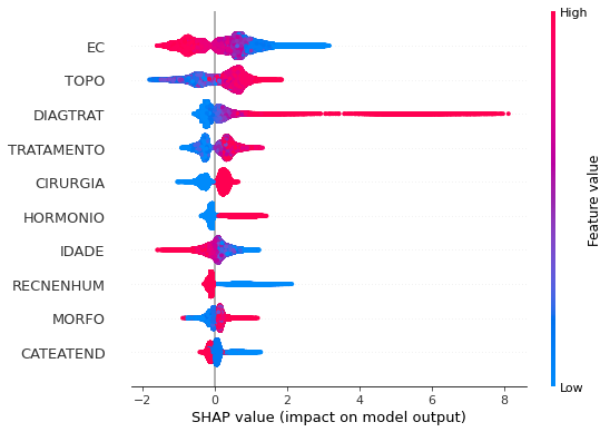
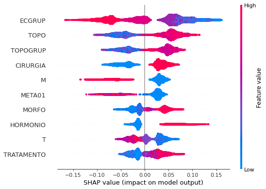
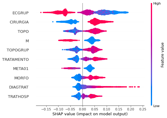
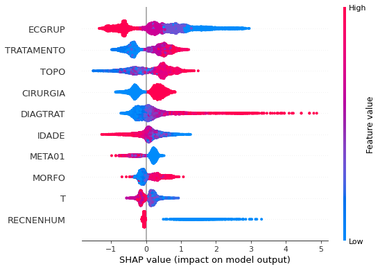
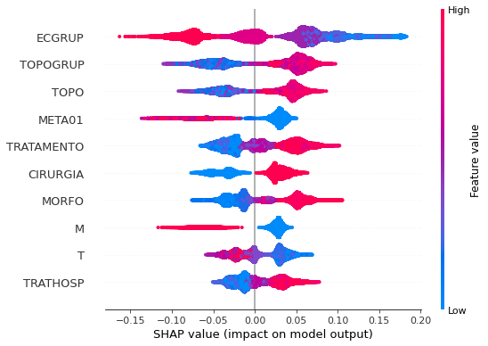
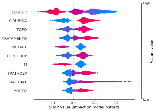
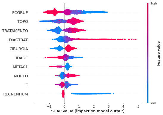
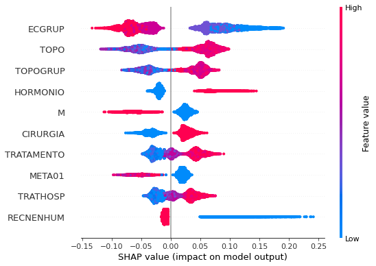
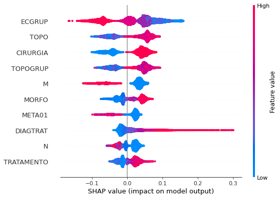
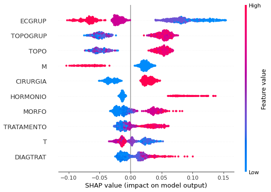
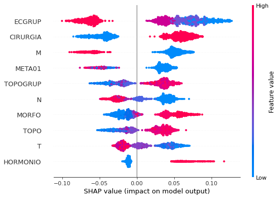
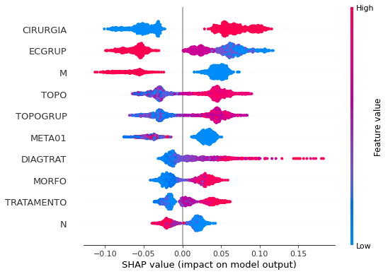
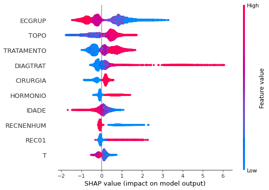
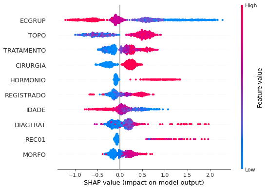
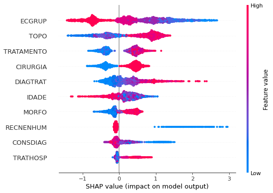
plot_shap_values(rf_sp, X_test_SP, feat_cols_SP)
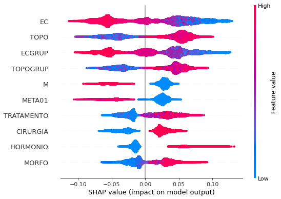
Note that larger values of the EC column, shown in pink, have more influence for the model’s prediction to be class 0, smaller values have greater weight for the prediction to be class 1.
The other columns shown follow the same logic.
[ ]:
# Other states
rf_fora = RandomForestClassifier(class_weight={0:6.42, 1:1},
                                 random_state=seed,
                                 criterion='entropy',
                                 max_depth=10)

rf_fora.fit(X_train_OS, y_train_OS)
RandomForestClassifier(class_weight={0: 6.42, 1: 1}, criterion='entropy',
                       max_depth=10, random_state=10)
[ ]:
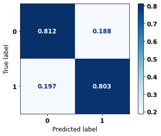
display_confusion_matrix(rf_fora, X_test_OS, y_test_OS)

              precision    recall  f1-score   support

           0      0.527     0.845     0.649      1266
           1      0.964     0.844     0.900      6177

    accuracy                          0.844      7443
   macro avg      0.745     0.845     0.774      7443
weighted avg      0.889     0.844     0.857      7443
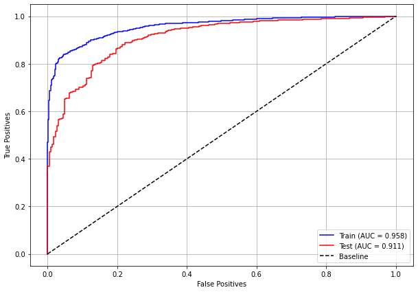
The confusion matrix obtained for the Random Forest algorithm, with other states data, shows a good performance of the model, because the model achieves a 84% of accuracy.
[ ]:
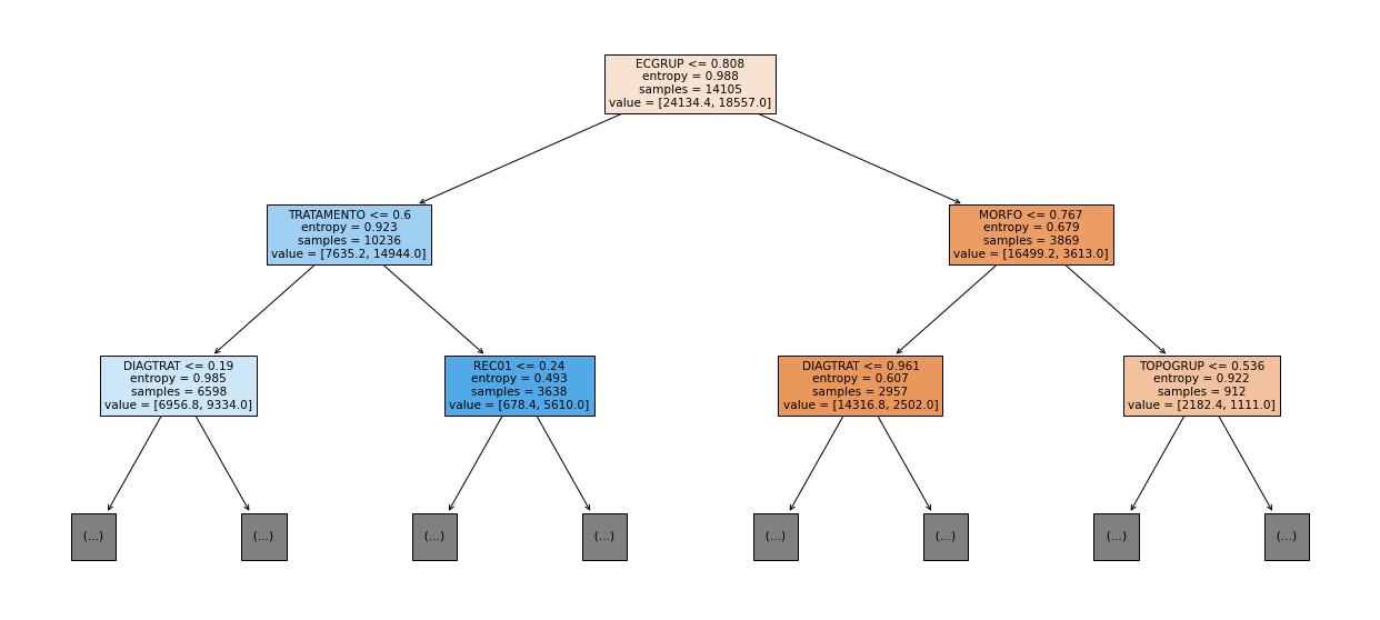
show_tree(rf_fora, feat_cols_OS, 2)
[ ]:
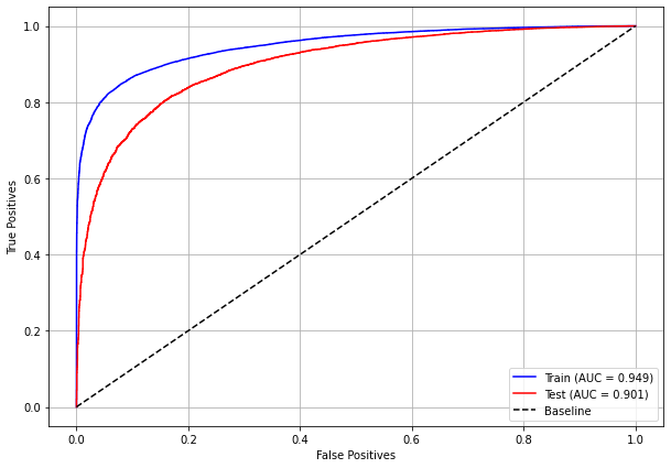
plot_roc_curve(rf_fora, X_train_OS, X_test_OS, y_train_OS, y_test_OS)

[ ]:
plot_feat_importances(rf_fora, feat_cols_OS)
The four most important features in the model were
ECGRUP,EC,TOPOandTOPOGRUP.
[ ]:
plot_shap_values(rf_fora, X_test_OS, feat_cols_OS)
Note that larger values of the ECGRUP column, shown in pink, have more influence for the model’s prediction to be class 0, smaller values have greater weight for the prediction to be class 1. This behavior was expected, because the higher the clinical stage, worse is the stage of cancer.
The other columns shown follow the same logic.
Randomized Grid Search
[ ]:
# RandomizedSearchCV
hyperRF = {'n_estimators': [100, 150, 200, 250],
           'max_depth': [5, 8, 10, 12, 15],
           'min_samples_split': [2, 5, 10, 15],
           'min_samples_leaf': [1, 2, 5, 10]}

rf = RandomForestClassifier(random_state=seed, criterion='entropy')

randRS = RandomizedSearchCV(rf, hyperRF, n_iter=20, cv=5, n_jobs=-1,
                            random_state=seed)
[ ]:
# SP
bestSP = randRS.fit(X_train_SP, y_train_SP)
[ ]:
bestSP.best_params_
{'n_estimators': 200,
 'min_samples_split': 10,
 'min_samples_leaf': 2,
 'max_depth': 15}
[ ]:
# SP
rf_sp_opt = bestSP.best_estimator_
rf_sp_opt.set_params(class_weight={0:5.15, 1:1})

rf_sp_opt.fit(X_train_SP, y_train_SP)
RandomForestClassifier(class_weight={0: 5.15, 1: 1}, criterion='entropy',
                       max_depth=15, min_samples_leaf=2, min_samples_split=10,
                       n_estimators=200, random_state=10)
[ ]:
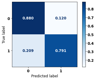
display_confusion_matrix(rf_sp_opt, X_test_SP, y_test_SP)

              precision    recall  f1-score   support

           0      0.530     0.831     0.647     21791
           1      0.956     0.832     0.890     95635

    accuracy                          0.832    117426
   macro avg      0.743     0.832     0.769    117426
weighted avg      0.877     0.832     0.845    117426
[ ]:
# Other States
bestOS = randRS.fit(X_train_OS, y_train_OS)
[ ]:
bestOS.best_params_
{'n_estimators': 200,
 'min_samples_split': 10,
 'min_samples_leaf': 2,
 'max_depth': 15}
[ ]:
# Other states
rf_fora_opt = bestOS.best_estimator_
rf_fora_opt.set_params(class_weight={0:17.7, 1:1})

rf_fora_opt.fit(X_train_OS, y_train_OS)
RandomForestClassifier(class_weight={0: 17.7, 1: 1}, criterion='entropy',
                       max_depth=15, min_samples_leaf=2, min_samples_split=10,
                       n_estimators=200, random_state=10)
[ ]:
display_confusion_matrix(rf_fora_opt, X_test_OS, y_test_OS)

              precision    recall  f1-score   support

           0      0.524     0.844     0.647      1266
           1      0.964     0.843     0.899      6177

    accuracy                          0.843      7443
   macro avg      0.744     0.844     0.773      7443
weighted avg      0.889     0.843     0.856      7443
XGBoost
The training of the XGBoost model follows the same pattern with random_state. A higher weight was also used for the class with fewer examples, using the hyperparameter scale_pos_weight.
The hyperparameter max_depth was chosen as 10 because the default value for this hyperparameter is 3, a low value for the amount of data we have.
[ ]:
# SP
xgboost_sp = XGBClassifier(max_depth=10,
                           scale_pos_weight=0.225,
                           random_state=seed)

xgboost_sp.fit(X_train_SP, y_train_SP)
XGBClassifier(max_depth=10, random_state=10, scale_pos_weight=0.225)
[ ]:
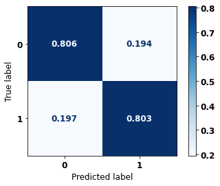
display_confusion_matrix(xgboost_sp, X_test_SP, y_test_SP)

              precision    recall  f1-score   support

           0      0.546     0.840     0.662     21791
           1      0.958     0.841     0.896     95635

    accuracy                          0.841    117426
   macro avg      0.752     0.840     0.779    117426
weighted avg      0.882     0.841     0.853    117426
The confusion matrix obtained for the XGBoost, with SP data, shows a good performance of the model, with 84% of accuracy.
[ ]:
plot_roc_curve(xgboost_sp, X_train_SP, X_test_SP, y_train_SP, y_test_SP)
[ ]:
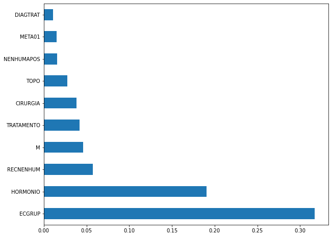
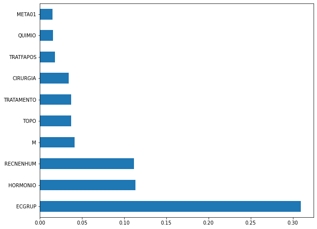
plot_feat_importances(xgboost_sp, feat_cols_SP)
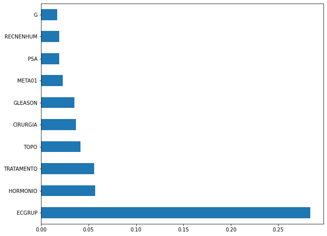
The four most important features in the model were
ECGRUP,EC,HORMONIOandRECNENHUM.
[ ]:
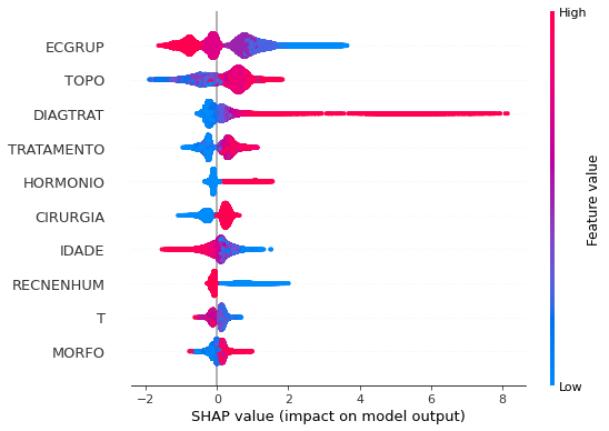
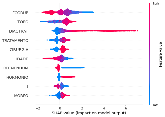
plot_shap_values(xgboost_sp, X_test_SP, feat_cols_SP)
Note that larger values of the EC column, shown in pink, have more influence for the model’s prediction to be class 0, smaller values have greater weight for the prediction to be class 1. This behavior was expected, because the higher the clinical stage, worse is the stage of cancer.
The other columns shown follow the same logic.
[ ]:
# Other states
xgboost_fora = XGBClassifier(max_depth=8,
                             scale_pos_weight=0.152,
                             random_state=seed)

xgboost_fora.fit(X_train_OS, y_train_OS)
XGBClassifier(max_depth=8, random_state=10, scale_pos_weight=0.152)
[ ]:
display_confusion_matrix(xgboost_fora, X_test_OS, y_test_OS)

              precision    recall  f1-score   support

           0      0.532     0.849     0.654      1266
           1      0.965     0.847     0.902      6177

    accuracy                          0.847      7443
   macro avg      0.748     0.848     0.778      7443
weighted avg      0.891     0.847     0.860      7443
The confusion matrix obtained for the XGBoost algorithm, with other states data, shows a good performance of the model, because the model achieves a 85% of accuracy.
[ ]:
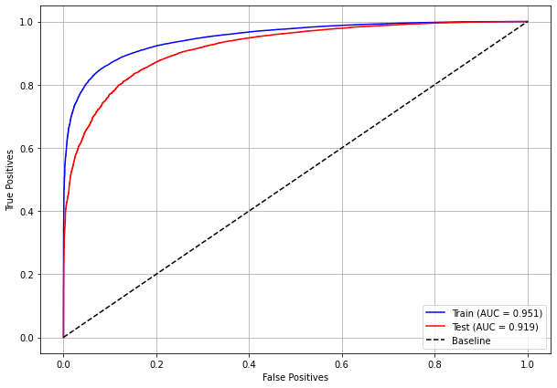
plot_roc_curve(xgboost_fora, X_train_OS, X_test_OS, y_train_OS, y_test_OS)

[ ]:
plot_feat_importances(xgboost_fora, feat_cols_OS)
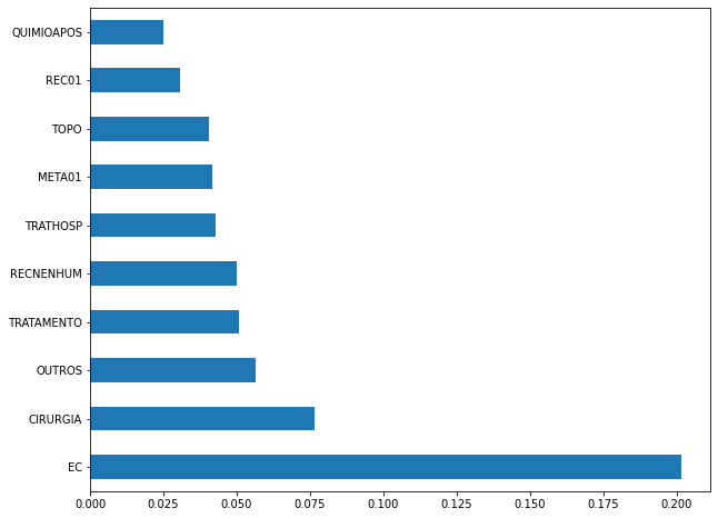
The four most important features in the model were
EC,CIRURGIA,OUTROSandTRATAMENTO.
[ ]:
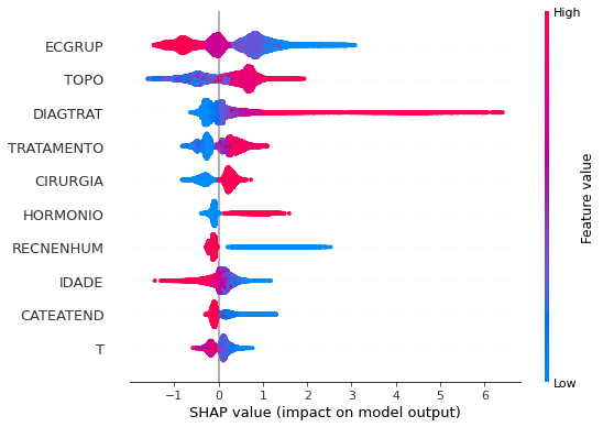
plot_shap_values(xgboost_fora, X_test_OS, feat_cols_OS)
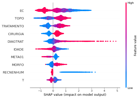
Note that larger values of the EC column, shown in pink, have more influence for the model’s prediction to be class 0, smaller values have greater weight for the prediction to be class 1. This behavior was expected, because the higher the clinical stage, worse is the stage of cancer.
The other columns shown follow the same logic.
Randomized Grid Search
[ ]:
# RandomizedSearchCV
hyperXGB = {'learning_rate': [0.05, 0.10, 0.15, 0.20],
            'max_depth': [5, 8, 10, 12, 15],
            'min_child_weight': [1, 3, 5, 7],
            'gamma': [0.0, 0.1, 0.2 , 0.3],
            'colsample_bytree': [0.3, 0.4, 0.5, 0.7],
            'n_estimators': [100, 150, 200, 250]}

xgboost = XGBClassifier(random_state=seed)
xgbRS = RandomizedSearchCV(xgboost, hyperXGB, n_iter=20, cv=5, n_jobs=-1,
                           random_state=seed)
[ ]:
# SP
bestSP = xgbRS.fit(X_train_SP, y_train_SP)
[ ]:
bestSP.best_params_
{'n_estimators': 200,
 'min_child_weight': 5,
 'max_depth': 10,
 'learning_rate': 0.1,
 'gamma': 0.2,
 'colsample_bytree': 0.4}
[ ]:
# SP
xgb_sp_opt = bestSP.best_estimator_
xgb_sp_opt.set_params(scale_pos_weight=0.224)

xgb_sp_opt.fit(X_train_SP, y_train_SP)
XGBClassifier(colsample_bytree=0.4, gamma=0.2, max_depth=10, min_child_weight=5,
              n_estimators=200, random_state=10, scale_pos_weight=0.224)
[ ]:
display_confusion_matrix(xgb_sp_opt, X_test_SP, y_test_SP)

              precision    recall  f1-score   support

           0      0.552     0.843     0.667     21791
           1      0.959     0.844     0.898     95635

    accuracy                          0.844    117426
   macro avg      0.756     0.844     0.783    117426
weighted avg      0.884     0.844     0.855    117426
[ ]:
# Other States
bestOS = xgbRS.fit(X_train_OS, y_train_OS)
[ ]:
bestOS.best_params_
{'n_estimators': 150,
 'min_child_weight': 5,
 'max_depth': 5,
 'learning_rate': 0.1,
 'gamma': 0.2,
 'colsample_bytree': 0.4}
[ ]:
# Other states
xgb_fora_opt = bestOS.best_estimator_
xgb_fora_opt.set_params(scale_pos_weight=0.206)

xgb_fora_opt.fit(X_train_OS, y_train_OS)
XGBClassifier(colsample_bytree=0.4, gamma=0.2, max_depth=5, min_child_weight=5,
              n_estimators=150, random_state=10, scale_pos_weight=0.206)
[ ]:
display_confusion_matrix(xgb_fora_opt, X_test_OS, y_test_OS)

              precision    recall  f1-score   support

           0      0.534     0.848     0.655      1266
           1      0.965     0.848     0.903      6177

    accuracy                          0.848      7443
   macro avg      0.749     0.848     0.779      7443
weighted avg      0.891     0.848     0.861      7443
Second approach
Approach without column EC as a feature.
Preprocessing
Now we are going to divide the data into training and testing, and then do the preprocessing in both datasets to perform the training of the models and their evaluation.
First, it is necessary to define the columns that will be used as features and the label. We will not use some columns of the datasets: UFRESID, because we already have the division between SP and other states in the two datasets.
It was chosen to keep the column IDADE, so we will not use the FAIXAETAR, as well as the column ECGRUP and not the column EC. Finally, the other columns contained in the list list_drop are possible labels, so they will not be used as features for machine learning models.
[ ]:
list_drop = ['UFRESID', 'FAIXAETAR', 'ULTICONS', 'ULTIDIAG', 'ULTITRAT',
             'obito_geral', 'obito_cancer', 'vivo_ano3', 'vivo_ano5',
             'ULTINFO', 'EC']

# 'RECNENHUM', 'RECLOCAL', 'RECREGIO', 'REC01', 'REC02', 'REC03', 'RECDIST'

lb = 'vivo_ano1'
A function was created to perform the preprocessing, preprocessing, that uses the other functions created, get_train_test (divides the dataset into train and test sets), train_preprocessing (do the preprocessing of the train set) and test_preprocessing (do the preprocessing of the test set).
To see the complete function go to the functions section.
SP
[ ]:
X_train_SP, X_test_SP, y_train_SP, y_test_SP, feat_cols_SP = preprocessing(df_SP_ano1, list_drop, lb,
                                                                           random_state=seed,
                                                                           balance_data=False,
                                                                           encoder_type='LabelEncoder',
                                                                           norm_name='StandardScaler')
X_train = (352278, 65), X_test = (117426, 65)
y_train = (352278,), y_test = (117426,)
Other states
[ ]:
X_train_OS, X_test_OS, y_train_OS, y_test_OS, feat_cols_OS = preprocessing(df_fora_ano1, list_drop, lb,
                                                                           random_state=seed,
                                                                           balance_data=False,
                                                                           encoder_type='LabelEncoder',
                                                                           norm_name='StandardScaler')
X_train = (22328, 65), X_test = (7443, 65)
y_train = (22328,), y_test = (7443,)
Training machine learning models
After dividing the data into training and testing, using the encoder and normalizing, the data is ready to be used by the machine learning models.
Random Forest
The first model that will be tested is the Random Forest, for this test the parameter random_state will be used, to obtain the same training values of the model every time it is runned.
The hyperparameter class_weight was also used, because the model has difficulty learning the class with fewer examples, so using this parameter this class will have a higher weight in the training of the model.
[ ]:
# SP
rf_sp = RandomForestClassifier(class_weight={0:4.23, 1:1},
                               random_state=seed,
                               criterion='entropy',
                               max_depth=10)

rf_sp.fit(X_train_SP, y_train_SP)
RandomForestClassifier(class_weight={0: 4.23, 1: 1}, criterion='entropy',
                       max_depth=10, random_state=10)
[ ]:
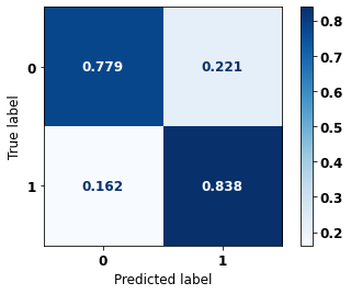
display_confusion_matrix(rf_sp, X_test_SP, y_test_SP)

              precision    recall  f1-score   support

           0      0.510     0.821     0.629     21791
           1      0.953     0.820     0.881     95635

    accuracy                          0.820    117426
   macro avg      0.731     0.821     0.755    117426
weighted avg      0.871     0.820     0.835    117426
The confusion matrix obtained for the Random Forest, with SP data, shows a good performance of the model, with 82% of accuracy.
[ ]:
show_tree(rf_sp, feat_cols_SP, 2)
[ ]:
plot_roc_curve(rf_sp, X_train_SP, X_test_SP, y_train_SP, y_test_SP)

[ ]:
plot_feat_importances(rf_sp, feat_cols_SP)
The four most important features in the model were
ECGRUP,TOPO,TOPOGRUPandM.
[ ]:
plot_shap_values(rf_sp, X_test_SP, feat_cols_SP)
Note that larger values of the ECGRUP column, shown in pink, have more influence for the model’s prediction to be class 0, smaller values have greater weight for the prediction to be class 1. This behavior was expected, because the higher the clinical stage, worse is the stage of cancer.
The other columns shown follow the same logic.
[ ]:
# Other states
rf_fora = RandomForestClassifier(class_weight={0:6.4, 1:1},
                                 random_state=seed,
                                 criterion='entropy',
                                 max_depth=10)

rf_fora.fit(X_train_OS, y_train_OS)
RandomForestClassifier(class_weight={0: 6.4, 1: 1}, criterion='entropy',
                       max_depth=10, random_state=10)
[ ]:
display_confusion_matrix(rf_fora, X_test_OS, y_test_OS)

              precision    recall  f1-score   support

           0      0.520     0.841     0.643      1266
           1      0.963     0.841     0.898      6177

    accuracy                          0.841      7443
   macro avg      0.741     0.841     0.770      7443
weighted avg      0.887     0.841     0.854      7443
The confusion matrix obtained for the Random Forest algorithm, with other states data, shows a good performance of the model, because the model achieves a 84% of accuracy.
[ ]:
show_tree(rf_fora, feat_cols_OS, 2)
[ ]:
plot_roc_curve(rf_fora, X_train_OS, X_test_OS, y_train_OS, y_test_OS)

[ ]:
plot_feat_importances(rf_fora, feat_cols_OS)
The four most important features in the model were
ECGRUP,TOPO,MandCIRURGIA.
[ ]:
plot_shap_values(rf_fora, X_test_OS, feat_cols_OS)
Note that larger values of the ECGRUP column, shown in pink, have more influence for the model’s prediction to be class 0, smaller values have greater weight for the prediction to be class 1. This behavior was expected, because the higher the clinical stage, worse is the stage of cancer.
The other columns shown follow the same logic.
XGBoost
The training of the XGBoost model follows the same pattern with random_state. A higher weight was also used for the class with fewer examples, using the hyperparameter scale_pos_weight.
The hyperparameter max_depth was chosen as 10 because the default value for this hyperparameter is 3, a low value for the amount of data we have.
[ ]:
# SP
xgboost_sp = XGBClassifier(max_depth=10,
                           scale_pos_weight=0.225,
                           random_state=seed)

xgboost_sp.fit(X_train_SP, y_train_SP)
XGBClassifier(max_depth=10, random_state=10, scale_pos_weight=0.225)
[ ]:
display_confusion_matrix(xgboost_sp, X_test_SP, y_test_SP)

              precision    recall  f1-score   support

           0      0.546     0.841     0.662     21791
           1      0.959     0.841     0.896     95635

    accuracy                          0.841    117426
   macro avg      0.753     0.841     0.779    117426
weighted avg      0.882     0.841     0.853    117426
The confusion matrix obtained for the XGBoost, with SP data, shows a good performance of the model, with 84% of accuracy.
[ ]:
plot_roc_curve(xgboost_sp, X_train_SP, X_test_SP, y_train_SP, y_test_SP)

[ ]:
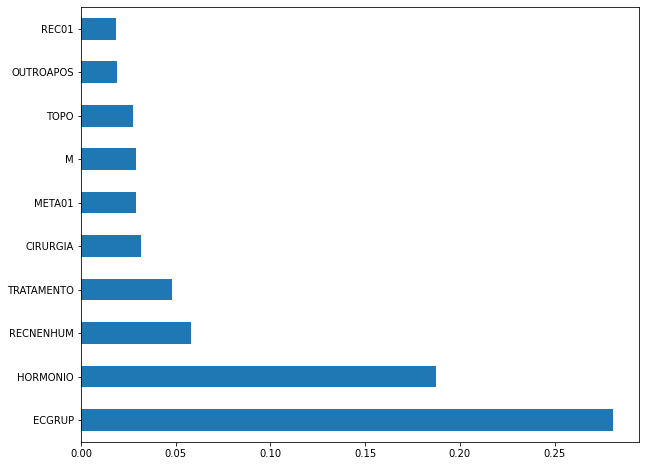
plot_feat_importances(xgboost_sp, feat_cols_SP)
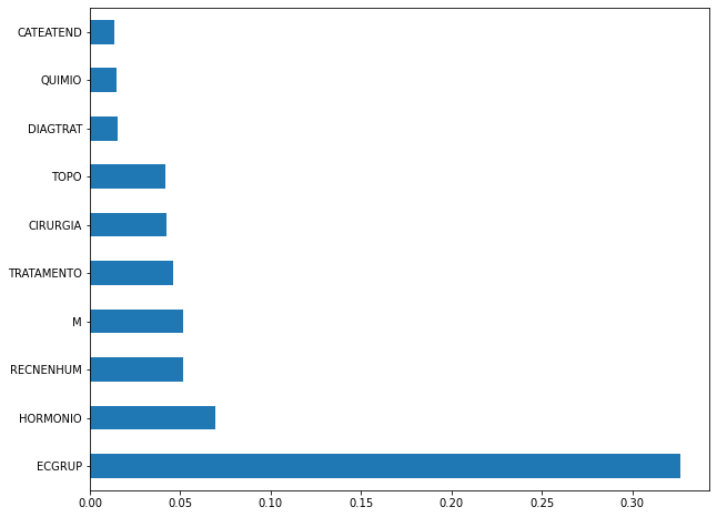
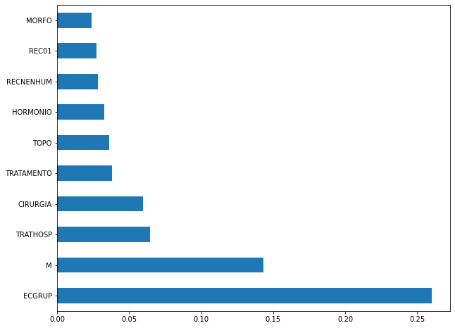
The four most important features in the model were
ECGRUP,HORMONIO,RECNENHUMandM.
[ ]:
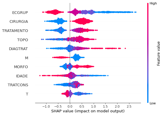
plot_shap_values(xgboost_sp, X_test_SP, feat_cols_SP)
Note that larger values of the ECGRUP column, shown in pink, have more influence for the model’s prediction to be class 0, smaller values have greater weight for the prediction to be class 1. This behavior was expected, because the higher the clinical stage, worse is the stage of cancer.
The other columns shown follow the same logic.
[ ]:
# Other states
xgboost_fora = XGBClassifier(max_depth=8,
                             scale_pos_weight=0.161,
                             random_state=seed)

xgboost_fora.fit(X_train_OS, y_train_OS)
XGBClassifier(max_depth=8, random_state=10, scale_pos_weight=0.161)
[ ]:
display_confusion_matrix(xgboost_fora, X_test_OS, y_test_OS)
              precision    recall  f1-score   support

           0      0.535     0.848     0.656      1266
           1      0.965     0.849     0.903      6177

    accuracy                          0.849      7443
   macro avg      0.750     0.849     0.780      7443
weighted avg      0.892     0.849     0.861      7443
The confusion matrix obtained for the XGBoost algorithm, with other states data, shows a good performance of the model, because the model achieves a 85% of accuracy.
[ ]:
plot_roc_curve(xgboost_fora, X_train_OS, X_test_OS, y_train_OS, y_test_OS)
[ ]:
plot_feat_importances(xgboost_fora, feat_cols_OS)
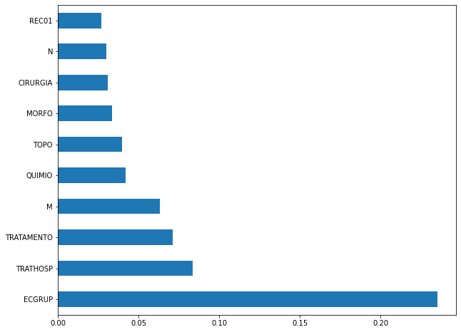
The four most important features in the model were
ECGRUP,CIRURGIA,TRATHOSPandTRATAMENTO.
[ ]:
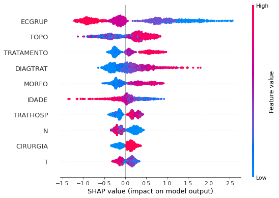
plot_shap_values(xgboost_fora, X_test_OS, feat_cols_OS)
Note that larger values of the ECGRUP column, shown in pink, have more influence for the model’s prediction to be class 0, smaller values have greater weight for the prediction to be class 1. This behavior was expected, because the higher the clinical stage, worse is the stage of cancer.
The other columns shown follow the same logic.
Third approach
Approach without column EC and HORMONIO as features.
Preprocessing
Now we are going to divide the data into training and testing, and then do the preprocessing in both datasets to perform the training of the models and their evaluation.
First, it is necessary to define the columns that will be used as features and the label. We will not use some columns of the datasets: UFRESID, because we already have the division between SP and other states in the two datasets.
It was chosen to keep the column IDADE, so we will not use the FAIXAETAR, as well as the column ECGRUP and not the column EC. Finally, the other columns contained in the list list_drop are possible labels, so they will not be used as features for machine learning models.
[ ]:
list_drop = ['UFRESID', 'FAIXAETAR', 'ULTICONS', 'ULTIDIAG', 'ULTITRAT',
             'obito_geral', 'obito_cancer', 'vivo_ano3', 'vivo_ano5',
             'ULTINFO', 'EC', 'HORMONIO']

# 'RECNENHUM', 'RECLOCAL', 'RECREGIO', 'REC01', 'REC02', 'REC03', 'RECDIST'

lb = 'vivo_ano1'
A function was created to perform the preprocessing, preprocessing, that uses the other functions created, get_train_test (divides the dataset into train and test sets), train_preprocessing (do the preprocessing of the train set) and test_preprocessing (do the preprocessing of the test set).
To see the complete function go to the functions section.
SP
[ ]:
X_train_SP, X_test_SP, y_train_SP, y_test_SP, feat_cols_SP = preprocessing(df_SP_ano1, list_drop, lb,
                                                                           random_state=seed,
                                                                           balance_data=False,
                                                                           encoder_type='LabelEncoder',
                                                                           norm_name='StandardScaler')
X_train = (352278, 64), X_test = (117426, 64)
y_train = (352278,), y_test = (117426,)
Other states
[ ]:
X_train_OS, X_test_OS, y_train_OS, y_test_OS, feat_cols_OS = preprocessing(df_fora_ano1, list_drop, lb,
                                                                           random_state=seed,
                                                                           balance_data=False,
                                                                           encoder_type='LabelEncoder',
                                                                           norm_name='StandardScaler')
X_train = (22328, 64), X_test = (7443, 64)
y_train = (22328,), y_test = (7443,)
Training machine learning models
After dividing the data into training and testing, using the encoder and normalizing, the data is ready to be used by the machine learning models.
Random Forest
The first model that will be tested is the Random Forest, for this test the parameter random_state will be used, to obtain the same training values of the model every time it is runned.
The hyperparameter class_weight was also used, because the model has difficulty learning the class with fewer examples, so using this parameter this class will have a higher weight in the training of the model.
[ ]:
# SP
rf_sp = RandomForestClassifier(class_weight={0:4.2, 1:1},
                               random_state=seed,
                               criterion='entropy',
                               max_depth=10)

rf_sp.fit(X_train_SP, y_train_SP)
RandomForestClassifier(class_weight={0: 4.2, 1: 1}, criterion='entropy',
                       max_depth=10, random_state=10)
[ ]:
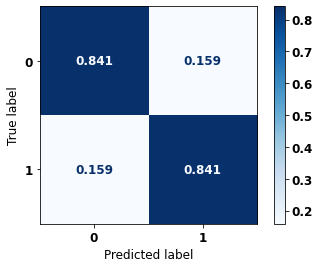
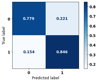
display_confusion_matrix(rf_sp, X_test_SP, y_test_SP)

              precision    recall  f1-score   support

           0      0.512     0.822     0.631     21791
           1      0.953     0.821     0.882     95635

    accuracy                          0.821    117426
   macro avg      0.732     0.822     0.756    117426
weighted avg      0.871     0.821     0.836    117426
The confusion matrix obtained for the Random Forest, with SP data, shows a good performance of the model, with 82% of accuracy.
[ ]:
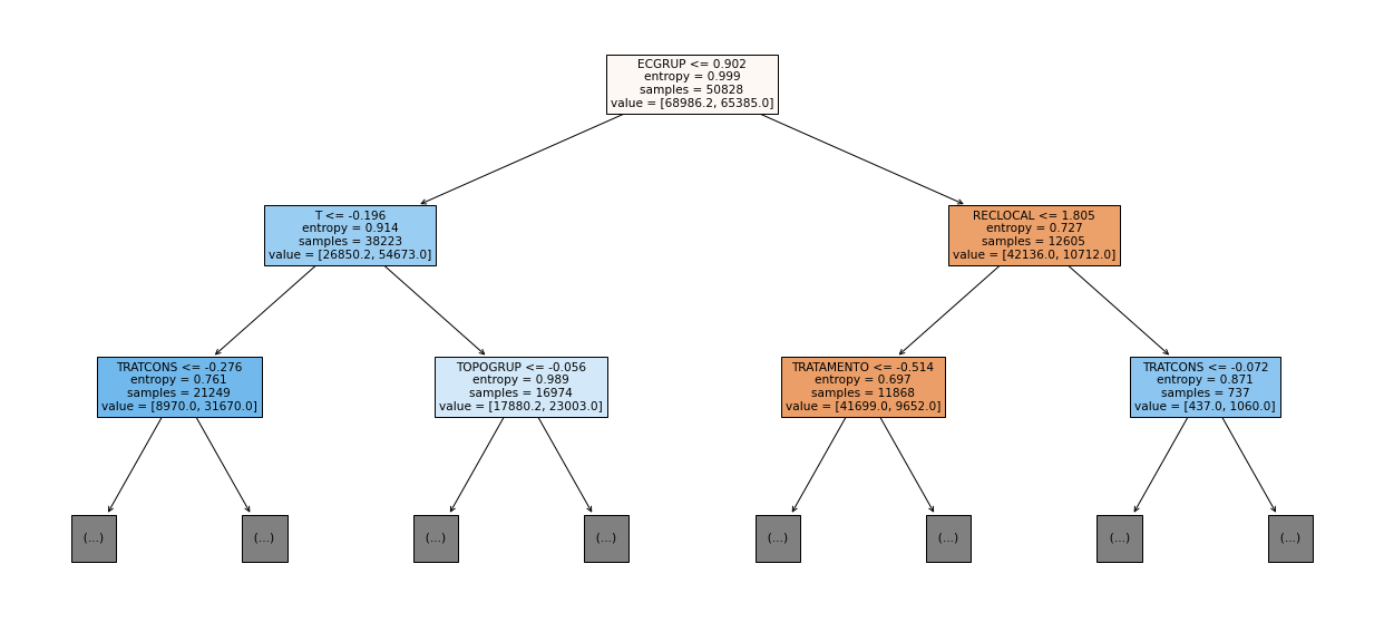
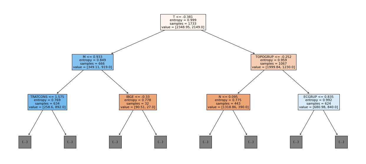
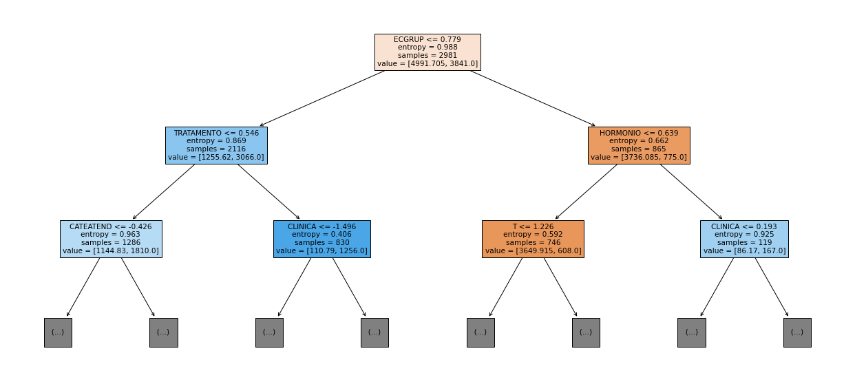
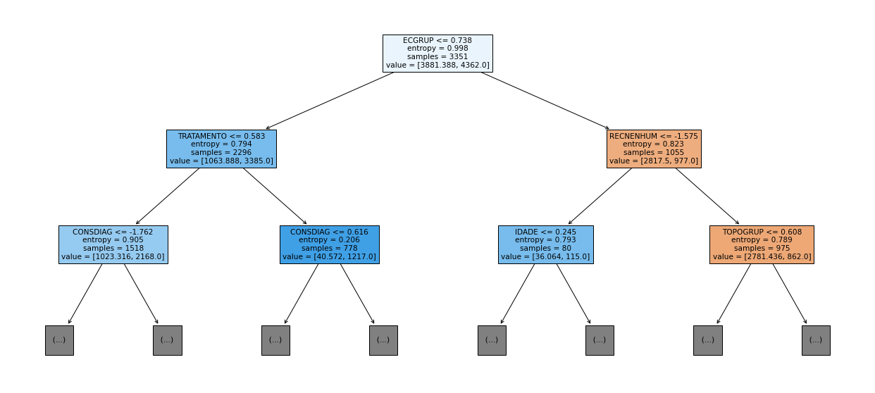
show_tree(rf_sp, feat_cols_SP, 2)
[ ]:
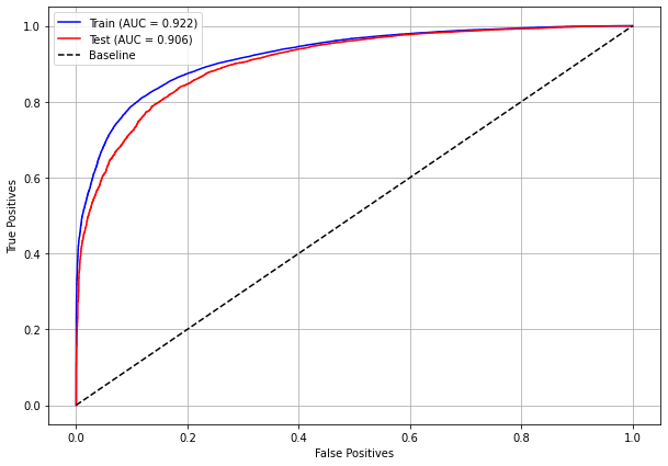
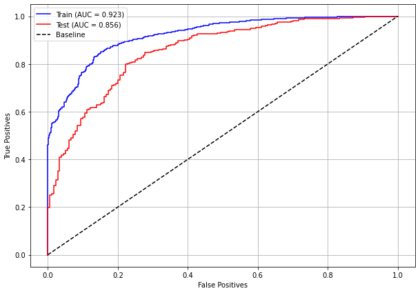
plot_roc_curve(rf_sp, X_train_SP, X_test_SP, y_train_SP, y_test_SP)
[ ]:
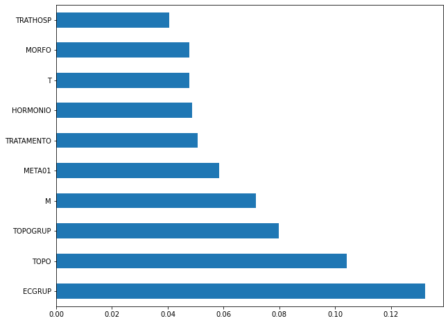
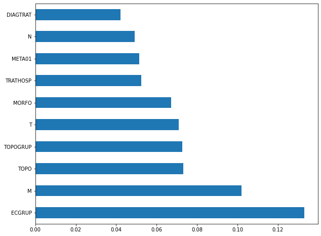
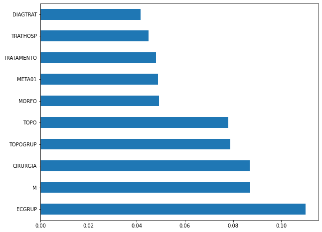
plot_feat_importances(rf_sp, feat_cols_SP)
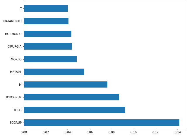
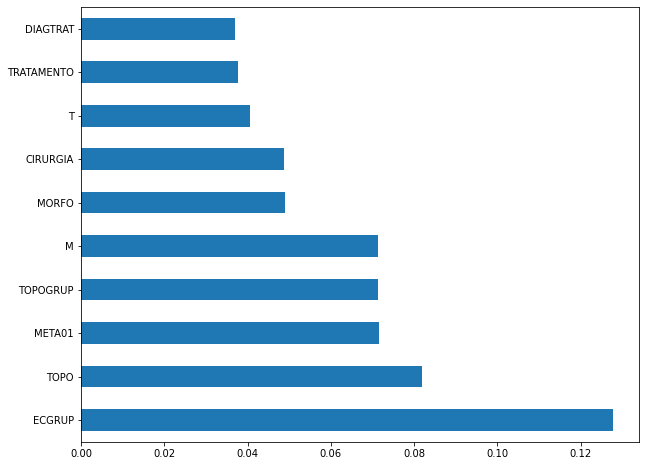
The four most important features in the model were
ECGRUP,TOPOGRUP,TOPOandMETA01.
[ ]:
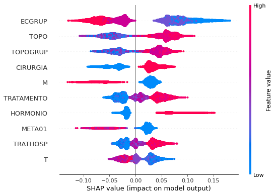
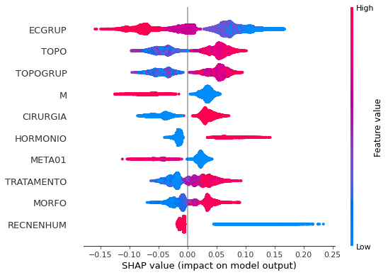
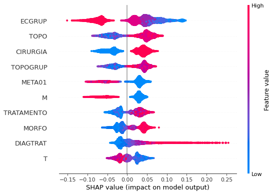
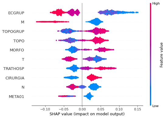
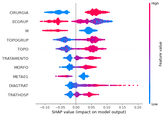
plot_shap_values(rf_sp, X_test_SP, feat_cols_SP)
Note that larger values of the ECGRUP column, shown in pink, have more influence for the model’s prediction to be class 0, smaller values have greater weight for the prediction to be class 1. This behavior was expected, because the higher the clinical stage, worse is the stage of cancer.
The other columns shown follow the same logic.
[ ]:
# Other states
rf_fora = RandomForestClassifier(class_weight={0:6.6, 1:1},
                                 random_state=seed,
                                 criterion='entropy',
                                 max_depth=10)

rf_fora.fit(X_train_OS, y_train_OS)
RandomForestClassifier(class_weight={0: 6.6, 1: 1}, criterion='entropy',
                       max_depth=10, random_state=10)
[ ]:
display_confusion_matrix(rf_fora, X_test_OS, y_test_OS)
              precision    recall  f1-score   support

           0      0.521     0.841     0.644      1266
           1      0.963     0.842     0.898      6177

    accuracy                          0.842      7443
   macro avg      0.742     0.841     0.771      7443
weighted avg      0.888     0.842     0.855      7443
The confusion matrix obtained for the Random Forest algorithm, with other states data, shows a good performance of the model, because the model achieves a 84% of accuracy.
[ ]:
show_tree(rf_fora, feat_cols_OS, 2)
[ ]:
plot_roc_curve(rf_fora, X_train_OS, X_test_OS, y_train_OS, y_test_OS)

[ ]:
plot_feat_importances(rf_fora, feat_cols_OS)
The four most important features in the model were
ECGRUP,TOPO,META01andTOPOGRUP.
[ ]:
plot_shap_values(rf_fora, X_test_OS, feat_cols_OS)
Note that larger values of the ECGRUP column, shown in pink, have more influence for the model’s prediction to be class 0, smaller values have greater weight for the prediction to be class 1. This behavior was expected, because the higher the clinical stage, worse is the stage of cancer.
The other columns shown follow the same logic.
XGBoost
The training of the XGBoost model follows the same pattern with random_state. A higher weight was also used for the class with fewer examples, using the hyperparameter scale_pos_weight.
The hyperparameter max_depth was chosen as 10 because the default value for this hyperparameter is 3, a low value for the amount of data we have.
[ ]:
# SP
xgboost_sp = XGBClassifier(max_depth=10,
                               scale_pos_weight=0.225,
                               random_state=seed)

xgboost_sp.fit(X_train_SP, y_train_SP)
XGBClassifier(max_depth=10, random_state=10, scale_pos_weight=0.225)
[ ]:
display_confusion_matrix(xgboost_sp, X_test_SP, y_test_SP)

              precision    recall  f1-score   support

           0      0.545     0.840     0.661     21791
           1      0.959     0.840     0.895     95635

    accuracy                          0.840    117426
   macro avg      0.752     0.840     0.778    117426
weighted avg      0.882     0.840     0.852    117426
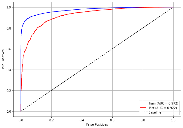
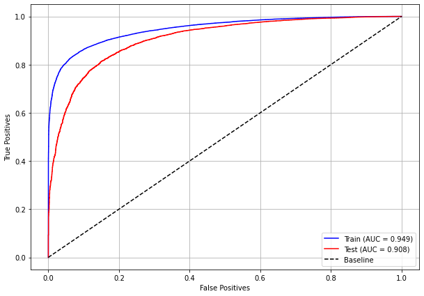
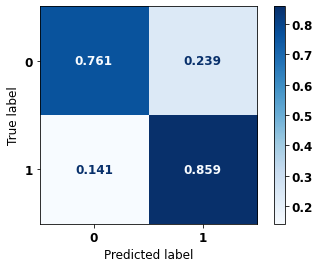
The confusion matrix obtained for the XGBoost, with SP data, shows a good performance of the model, with 84% of accuracy.
[ ]:
plot_roc_curve(xgboost_sp, X_train_SP, X_test_SP, y_train_SP, y_test_SP)

[ ]:
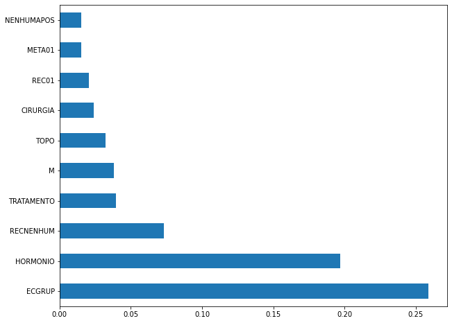
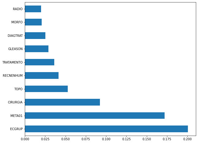
plot_feat_importances(xgboost_sp, feat_cols_SP)
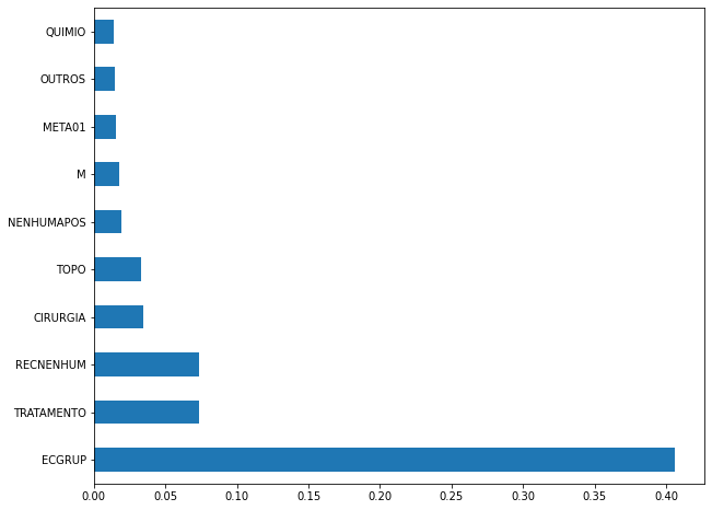
The four most important features in the model were
ECGRUP,TRATAMENTO,RECNENHUMandCIRURGIA.
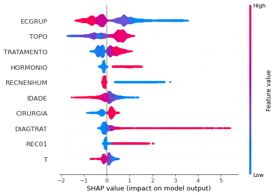
[ ]:
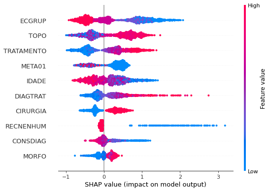
plot_shap_values(xgboost_sp, X_test_SP, feat_cols_SP)
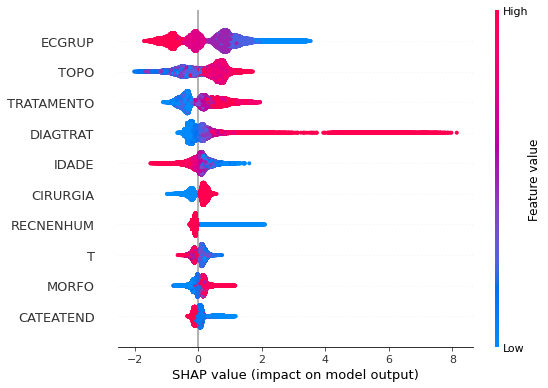
Note that larger values of the ECGRUP column, shown in pink, have more influence for the model’s prediction to be class 0, smaller values have greater weight for the prediction to be class 1. This behavior was expected, because the higher the clinical stage, worse is the stage of cancer.
The other columns shown follow the same logic.
[ ]:
# Other states
xgboost_fora = XGBClassifier(max_depth=8,
                             scale_pos_weight=0.156,
                             random_state=seed)

xgboost_fora.fit(X_train_OS, y_train_OS)
XGBClassifier(max_depth=8, random_state=10, scale_pos_weight=0.156)
[ ]:
display_confusion_matrix(xgboost_fora, X_test_OS, y_test_OS)

              precision    recall  f1-score   support

           0      0.532     0.847     0.653      1266
           1      0.964     0.847     0.902      6177

    accuracy                          0.847      7443
   macro avg      0.748     0.847     0.778      7443
weighted avg      0.891     0.847     0.860      7443
The confusion matrix obtained for the XGBoost algorithm, with other states data, shows a good performance of the model, because the model achieves a 85% of accuracy.
[ ]:
plot_roc_curve(xgboost_fora, X_train_OS, X_test_OS, y_train_OS, y_test_OS)
[ ]:
plot_feat_importances(xgboost_fora, feat_cols_OS)
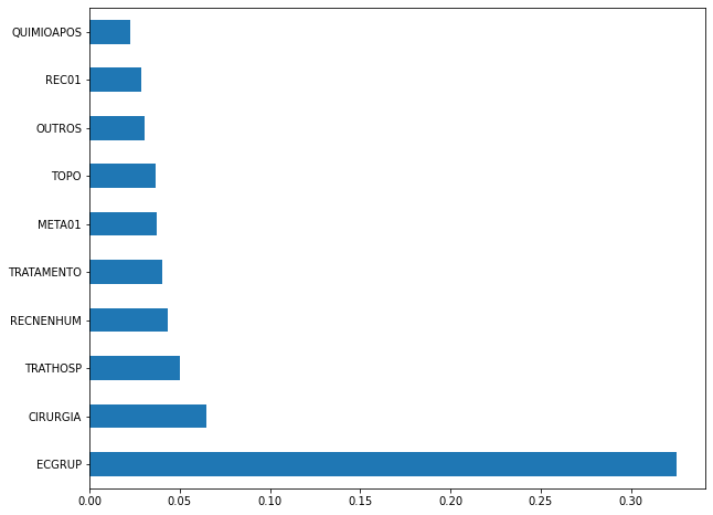
The four most important features in the model were
ECGRUP,CIRURGIA,TRATHOSPandRECNENHUM.
[ ]:
plot_shap_values(xgboost_fora, X_test_OS, feat_cols_OS)
Note that larger values of the ECGRUP column, shown in pink, have more influence for the model’s prediction to be class 0, smaller values have greater weight for the prediction to be class 1. This behavior was expected, because the higher the clinical stage, worse is the stage of cancer.
The other columns shown follow the same logic.
Fourth approach
Approach with grouped years and without the column EC.
Preprocessing
Now we are going to divide the data into training and testing, and then do the preprocessing in both datasets to perform the training of the models and their evaluation. We will use the years grouped too, resulting in 5 datasets for SP and more 5 for other states.
First, it is necessary to define the columns that will be used as features and the label. We will not use some columns of the datasets: UFRESID, because we already have the division between SP and other states in the two datasets.
It was chosen to keep the column IDADE, so we will not use the FAIXAETAR, as well as the column ECGRUP and not the column EC. Finally, the other columns contained in the list list_drop are possible labels, so they will not be used as features for machine learning models.
[ ]:
list_drop = ['UFRESID', 'FAIXAETAR', 'ULTICONS', 'ULTIDIAG', 'ULTITRAT',
             'obito_geral', 'obito_cancer', 'vivo_ano3', 'vivo_ano5', 'ULTINFO',
             'EC']

# 'RECNENHUM', 'RECLOCAL', 'RECREGIO', 'REC01', 'REC02', 'REC03', 'RECDIST'

lb = 'vivo_ano1'
A function was created to perform the preprocessing, preprocessing, that uses the other functions created, get_train_test (divides the dataset into train and test sets), train_preprocessing (do the preprocessing of the train set) and test_preprocessing (do the preprocessing of the test set).
The process will be done 5 times for SP and other states, using the datasets with grouped years.
To see the complete function go to the functions section.
SP
[ ]:
X_trainSP_00_03, X_testSP_00_03, y_trainSP_00_03, y_testSP_00_03, feat_SP_00_03 = preprocessing(df_SP_ano1, list_drop, lb,
                                                                                                group_years=True,
                                                                                                first_year=2000,
                                                                                                last_year=2003,
                                                                                                random_state=seed,
                                                                                                balance_data=False,
                                                                                                encoder_type='LabelEncoder',
                                                                                                norm_name='StandardScaler')
X_train = (47196, 65), X_test = (15732, 65)
y_train = (47196,), y_test = (15732,)
[ ]:
X_trainSP_04_07, X_testSP_04_07, y_trainSP_04_07, y_testSP_04_07, feat_SP_04_07 = preprocessing(df_SP_ano1, list_drop, lb,
                                                                                                group_years=True,
                                                                                                first_year=2004,
                                                                                                last_year=2007,
                                                                                                random_state=seed,
                                                                                                balance_data=False,
                                                                                                encoder_type='LabelEncoder',
                                                                                                norm_name='StandardScaler')
X_train = (59781, 65), X_test = (19928, 65)
y_train = (59781,), y_test = (19928,)
[ ]:
X_trainSP_08_11, X_testSP_08_11, y_trainSP_08_11, y_testSP_08_11, feat_SP_08_11 = preprocessing(df_SP_ano1, list_drop, lb,
                                                                                                group_years=True,
                                                                                                first_year=2008,
                                                                                                last_year=2011,
                                                                                                random_state=seed,
                                                                                                balance_data=False,
                                                                                                encoder_type='LabelEncoder',
                                                                                                norm_name='StandardScaler')
X_train = (80382, 65), X_test = (26795, 65)
y_train = (80382,), y_test = (26795,)
[ ]:
X_trainSP_12_15, X_testSP_12_15, y_trainSP_12_15, y_testSP_12_15, feat_SP_12_15 = preprocessing(df_SP_ano1, list_drop, lb,
                                                                                                group_years=True,
                                                                                                first_year=2012,
                                                                                                last_year=2015,
                                                                                                random_state=seed,
                                                                                                balance_data=False,
                                                                                                encoder_type='LabelEncoder',
                                                                                                norm_name='StandardScaler')
X_train = (99850, 65), X_test = (33284, 65)
y_train = (99850,), y_test = (33284,)
[ ]:
X_trainSP_16_21, X_testSP_16_21, y_trainSP_16_21, y_testSP_16_21, feat_SP_16_21 = preprocessing(df_SP_ano1, list_drop, lb,
                                                                                                group_years=True,
                                                                                                first_year=2016,
                                                                                                last_year=2021,
                                                                                                random_state=seed,
                                                                                                balance_data=False,
                                                                                                encoder_type='LabelEncoder',
                                                                                                norm_name='StandardScaler')
X_train = (65067, 65), X_test = (21689, 65)
y_train = (65067,), y_test = (21689,)
Other states
[ ]:
X_trainOS_00_03, X_testOS_00_03, y_trainOS_00_03, y_testOS_00_03, feat_OS_00_03 = preprocessing(df_fora_ano1, list_drop, lb,
                                                                                                group_years=True,
                                                                                                first_year=2000,
                                                                                                last_year=2003,
                                                                                                random_state=seed,
                                                                                                balance_data=False,
                                                                                                encoder_type='LabelEncoder',
                                                                                                norm_name='StandardScaler')
X_train = (2694, 65), X_test = (899, 65)
y_train = (2694,), y_test = (899,)
[ ]:
X_trainOS_04_07, X_testOS_04_07, y_trainOS_04_07, y_testOS_04_07, feat_OS_04_07 = preprocessing(df_fora_ano1, list_drop, lb,
                                                                                                group_years=True,
                                                                                                first_year=2004,
                                                                                                last_year=2007,
                                                                                                random_state=seed,
                                                                                                balance_data=False,
                                                                                                encoder_type='LabelEncoder',
                                                                                                norm_name='StandardScaler')
X_train = (3738, 65), X_test = (1246, 65)
y_train = (3738,), y_test = (1246,)
[ ]:
X_trainOS_08_11, X_testOS_08_11, y_trainOS_08_11, y_testOS_08_11, feat_OS_08_11 = preprocessing(df_fora_ano1, list_drop, lb,
                                                                                                group_years=True,
                                                                                                first_year=2008,
                                                                                                last_year=2011,
                                                                                                random_state=seed,
                                                                                                balance_data=False,
                                                                                                encoder_type='LabelEncoder',
                                                                                                norm_name='StandardScaler')
X_train = (4652, 65), X_test = (1551, 65)
y_train = (4652,), y_test = (1551,)
[ ]:
X_trainOS_12_15, X_testOS_12_15, y_trainOS_12_15, y_testOS_12_15, feat_OS_12_15 = preprocessing(df_fora_ano1, list_drop, lb,
                                                                                                group_years=True,
                                                                                                first_year=2012,
                                                                                                last_year=2015,
                                                                                                random_state=seed,
                                                                                                balance_data=False,
                                                                                                encoder_type='LabelEncoder',
                                                                                                norm_name='StandardScaler')
X_train = (6019, 65), X_test = (2007, 65)
y_train = (6019,), y_test = (2007,)
[ ]:
X_trainOS_16_20, X_testOS_16_20, y_trainOS_16_20, y_testOS_16_20, feat_OS_16_20 = preprocessing(df_fora_ano1, list_drop, lb,
                                                                                                group_years=True,
                                                                                                first_year=2016,
                                                                                                last_year=2020,
                                                                                                random_state=seed,
                                                                                                balance_data=False,
                                                                                                encoder_type='LabelEncoder',
                                                                                                norm_name='StandardScaler')
X_train = (5223, 65), X_test = (1742, 65)
y_train = (5223,), y_test = (1742,)
Training and evaluation of the models
After dividing the data into training and testing, using the encoder and normalizing, the data is ready to be used by the machine learning models.
Random Forest
The first model is the Random Forest, the random_state will be used as a parameter, to obtain the same training values of the model every time it is runned.
The hyperparameter class_weight was used because the models have difficulty to learn the class with fewer examples.
SP
[ ]:
# SP - 2000 to 2003
rf_sp_00_03 = RandomForestClassifier(random_state=seed,
                                     class_weight={0:3.58, 1:1},
                                     criterion='entropy',
                                     max_depth=10)

rf_sp_00_03.fit(X_trainSP_00_03, y_trainSP_00_03)
RandomForestClassifier(class_weight={0: 3.58, 1: 1}, criterion='entropy',
                       max_depth=10, random_state=10)
[ ]:
display_confusion_matrix(rf_sp_00_03, X_testSP_00_03, y_testSP_00_03)
              precision    recall  f1-score   support

           0      0.537     0.807     0.645      3430
           1      0.937     0.806     0.867     12302

    accuracy                          0.806     15732
   macro avg      0.737     0.806     0.756     15732
weighted avg      0.850     0.806     0.818     15732
The confusion matrix obtained for the Random Forest, with SP data from 2000 to 2003, shows a good performance of the model, with 81% of accuracy.
[ ]:
show_tree(rf_sp_00_03, feat_SP_00_03, 2)
[ ]:
plot_roc_curve(rf_sp_00_03, X_trainSP_00_03, X_testSP_00_03, y_trainSP_00_03, y_testSP_00_03)
[ ]:
plot_feat_importances(rf_sp_00_03, feat_SP_00_03)
The four most important features in the model were
ECGRUP,TOPO,TOPOGRUP, andM.
[ ]:
plot_shap_values(rf_sp_00_03, X_testSP_00_03, feat_SP_00_03)
Note that larger values of the ECGRUP column, shown in pink, have more influence for the model’s prediction to be class 0, smaller values have greater weight for the prediction to be class 1. This behavior was expected, because the higher the clinical stage, worse is the stage of cancer.
The other columns shown follow the same logic.
[ ]:
# SP - 2004 to 2007
rf_sp_04_07 = RandomForestClassifier(random_state=seed,
                                     class_weight={0:4.4, 1:1},
                                     criterion='entropy',
                                     max_depth=10)

rf_sp_04_07.fit(X_trainSP_04_07, y_trainSP_04_07)
RandomForestClassifier(class_weight={0: 4.4, 1: 1}, criterion='entropy',
                       max_depth=10, random_state=10)
[ ]:
display_confusion_matrix(rf_sp_04_07, X_testSP_04_07, y_testSP_04_07)

              precision    recall  f1-score   support

           0      0.534     0.822     0.647      3955
           1      0.949     0.822     0.881     15973

    accuracy                          0.822     19928
   macro avg      0.742     0.822     0.764     19928
weighted avg      0.867     0.822     0.835     19928
The confusion matrix obtained for the Random Forest, with SP data from 2004 to 2007, shows a good performance of the model, with 82% of accuracy.
[ ]:
show_tree(rf_sp_04_07, feat_SP_04_07, 2)
[ ]:
plot_roc_curve(rf_sp_04_07, X_trainSP_04_07, X_testSP_04_07, y_trainSP_04_07, y_testSP_04_07)
[ ]:
plot_feat_importances(rf_sp_04_07, feat_SP_04_07)
The four most important features in the model were
ECGRUP,TOPO,TOPOGRUPandM.
[ ]:
plot_shap_values(rf_sp_04_07, X_testSP_04_07, feat_SP_04_07)
Note that larger values of the ECGRUP column, shown in pink, have more influence for the model’s prediction to be class 0, smaller values have greater weight for the prediction to be class 1. This behavior was expected, because the higher the clinical stage, worse is the stage of cancer.
The other columns shown follow the same logic.
[ ]:
# SP - 2008 to 2011
rf_sp_08_11 = RandomForestClassifier(random_state=seed,
                                     class_weight={0:4.6, 1:1},
                                     criterion='entropy',
                                     max_depth=10)

rf_sp_08_11.fit(X_trainSP_08_11, y_trainSP_08_11)
RandomForestClassifier(class_weight={0: 4.6, 1: 1}, criterion='entropy',
                       max_depth=10, random_state=10)
[ ]:
display_confusion_matrix(rf_sp_08_11, X_testSP_08_11, y_testSP_08_11)

              precision    recall  f1-score   support

           0      0.520     0.825     0.638      5020
           1      0.953     0.825     0.884     21775

    accuracy                          0.825     26795
   macro avg      0.737     0.825     0.761     26795
weighted avg      0.872     0.825     0.838     26795
The confusion matrix obtained for the Random Forest, with SP data from 2008 to 2011, shows a good performance of the model, with 82% of accuracy.
[ ]:
show_tree(rf_sp_08_11, feat_SP_08_11, 2)
[ ]:
plot_roc_curve(rf_sp_08_11, X_trainSP_08_11, X_testSP_08_11, y_trainSP_08_11, y_testSP_08_11)
[ ]:
plot_feat_importances(rf_sp_08_11, feat_SP_08_11)
The four most important features in the model were
ECGRUP,TOPO,TOPOGRUPandM.
[ ]:
plot_shap_values(rf_sp_08_11, X_testSP_08_11, feat_SP_08_11)
Note that larger values of the ECGRUP column, shown in pink, have more influence for the model’s prediction to be class 0, smaller values have greater weight for the prediction to be class 1. This behavior was expected, because the higher the clinical stage, worse is the stage of cancer.
The other columns shown follow the same logic.
[ ]:
# SP - 2012 to 2015
rf_sp_12_15 = RandomForestClassifier(random_state=seed,
                                     class_weight={0:5.45, 1:1},
                                     criterion='entropy',
                                     max_depth=10)

rf_sp_12_15.fit(X_trainSP_12_15, y_trainSP_12_15)
RandomForestClassifier(class_weight={0: 5.45, 1: 1}, criterion='entropy',
                       max_depth=10, random_state=10)
[ ]:
display_confusion_matrix(rf_sp_12_15, X_testSP_12_15, y_testSP_12_15)

              precision    recall  f1-score   support

           0      0.482     0.827     0.609      5442
           1      0.961     0.826     0.888     27842

    accuracy                          0.826     33284
   macro avg      0.721     0.827     0.749     33284
weighted avg      0.882     0.826     0.843     33284
The confusion matrix obtained for the Random Forest, with SP data from 2012 to 2015, shows a good performance of the model with 83% of accuracy.
[ ]:
show_tree(rf_sp_12_15, feat_SP_12_15, 2)
[ ]:
plot_roc_curve(rf_sp_12_15, X_trainSP_12_15, X_testSP_12_15, y_trainSP_12_15, y_testSP_12_15)
[ ]:
plot_feat_importances(rf_sp_12_15, feat_SP_12_15)
The four most important features in the model were
ECGRUP,TOPO,TOPOGRUPandM.
[ ]:
plot_shap_values(rf_sp_12_15, X_testSP_12_15, feat_SP_12_15)
Note that larger values of the ECGRUP column, shown in pink, have more influence for the model’s prediction to be class 0, smaller values have greater weight for the prediction to be class 1. This behavior was expected, because the higher the clinical stage, worse is the stage of cancer.
The other columns shown follow the same logic.
[ ]:
# SP - 2016 to 2021
rf_sp_16_21 = RandomForestClassifier(random_state=seed,
                                     class_weight={0:4.6, 1:1},
                                     criterion='entropy',
                                     max_depth=10)

rf_sp_16_21.fit(X_trainSP_16_21, y_trainSP_16_21)
RandomForestClassifier(class_weight={0: 4.6, 1: 1}, criterion='entropy',
                       max_depth=10, random_state=10)
[ ]:
display_confusion_matrix(rf_sp_16_21, X_testSP_16_21, y_testSP_16_21)

              precision    recall  f1-score   support

           0      0.499     0.816     0.619      3944
           1      0.952     0.817     0.880     17745

    accuracy                          0.817     21689
   macro avg      0.725     0.817     0.749     21689
weighted avg      0.870     0.817     0.832     21689
The confusion matrix obtained for the Random Forest, with SP data from 2016 to 2021, shows a good performance of the model, with 82% of accuracy.
[ ]:
show_tree(rf_sp_16_21, feat_SP_16_21, 2)
[ ]:
plot_roc_curve(rf_sp_16_21, X_trainSP_16_21, X_testSP_16_21, y_trainSP_16_21, y_testSP_16_21)
[ ]:
plot_feat_importances(rf_sp_16_21, feat_SP_16_21)
The four most important features in the model were
ECGRUP,TOPO,META01, andTOPOGRUP.
[ ]:
plot_shap_values(rf_sp_16_21, X_testSP_16_21, feat_SP_16_21)
Note that larger values of the ECGRUP column, shown in pink, have more influence for the model’s prediction to be class 0, smaller values have greater weight for the prediction to be class 1. This behavior was expected, because the higher the clinical stage, worse is the stage of cancer.
The other columns shown follow the same logic.
Other states
[ ]:
# Other states - 2000 to 2003
rf_fora_00_03 = RandomForestClassifier(random_state=seed,
                                       class_weight={0:4.31, 1:1},
                                       criterion='entropy',
                                       max_depth=6)

rf_fora_00_03.fit(X_trainOS_00_03, y_trainOS_00_03)
RandomForestClassifier(class_weight={0: 4.31, 1: 1}, criterion='entropy',
                       max_depth=6, random_state=10)
[ ]:
display_confusion_matrix(rf_fora_00_03, X_testOS_00_03, y_testOS_00_03)

              precision    recall  f1-score   support

           0      0.467     0.778     0.583       180
           1      0.933     0.777     0.848       719

    accuracy                          0.778       899
   macro avg      0.700     0.778     0.716       899
weighted avg      0.840     0.778     0.795       899
The confusion matrix obtained for the Random Forest, with other states data from 2000 to 2003, also shows a good performance of the model, and we have a balanced main diagonal with 78% of accuracy.
[ ]:
show_tree(rf_fora_00_03, feat_OS_00_03, 2)
[ ]:
plot_roc_curve(rf_fora_00_03, X_trainOS_00_03, X_testOS_00_03, y_trainOS_00_03, y_testOS_00_03)
[ ]:
plot_feat_importances(rf_fora_00_03, feat_OS_00_03)
The four most important features in the model were
ECGRUP,TOPO,TOPOGRUPandM.
[ ]:
plot_shap_values(rf_fora_00_03, X_testOS_00_03, feat_OS_00_03)
Note that larger values of the ECGRUP column, shown in pink, have more influence for the model’s prediction to be class 0, smaller values have greater weight for the prediction to be class 1. This behavior was expected, because the higher the clinical stage, worse is the stage of cancer.
The other columns shown follow the same logic.
[ ]:
# Other states - 2004 to 2007
rf_fora_04_07 = RandomForestClassifier(random_state=seed,
                                       class_weight={0:4.807, 1:1},
                                       criterion='entropy',
                                       max_depth=6)

rf_fora_04_07.fit(X_trainOS_04_07, y_trainOS_04_07)
RandomForestClassifier(class_weight={0: 4.807, 1: 1}, criterion='entropy',
                       max_depth=6, random_state=10)
[ ]:
display_confusion_matrix(rf_fora_04_07, X_testOS_04_07, y_testOS_04_07)

              precision    recall  f1-score   support

           0      0.483     0.809     0.605       225
           1      0.951     0.809     0.874      1021

    accuracy                          0.809      1246
   macro avg      0.717     0.809     0.739      1246
weighted avg      0.866     0.809     0.825      1246
The confusion matrix obtained for the Random Forest, with other states data from 2004 to 2007, also shows a good performance of the model, with 81% of accuracy.
[ ]:
show_tree(rf_fora_04_07, feat_OS_04_07, 2)
[ ]:
plot_roc_curve(rf_fora_04_07, X_trainOS_04_07, X_testOS_04_07, y_trainOS_04_07, y_testOS_04_07)
[ ]:
plot_feat_importances(rf_fora_04_07, feat_OS_04_07)
The four most important features in the model were
ECGRUP,M,TOPOandTOPOGRUP.
[ ]:
plot_shap_values(rf_fora_04_07, X_testOS_04_07, feat_OS_04_07)
Note that larger values of the ECGRUP column, shown in pink, have more influence for the model’s prediction to be class 0, smaller values have greater weight for the prediction to be class 1. This behavior was expected, because the higher the clinical stage, worse is the stage of cancer.
The other columns shown follow the same logic.
[ ]:
# Other states - 2008 to 2011
rf_fora_08_11 = RandomForestClassifier(random_state=seed,
                                       class_weight={0:6.155, 1:1},
                                       criterion='entropy',
                                       max_depth=6)

rf_fora_08_11.fit(X_trainOS_08_11, y_trainOS_08_11)
RandomForestClassifier(class_weight={0: 6.155, 1: 1}, criterion='entropy',
                       max_depth=6, random_state=10)
[ ]:
display_confusion_matrix(rf_fora_08_11, X_testOS_08_11, y_testOS_08_11)
              precision    recall  f1-score   support

           0      0.521     0.841     0.643       264
           1      0.963     0.841     0.898      1287

    accuracy                          0.841      1551
   macro avg      0.742     0.841     0.771      1551
weighted avg      0.888     0.841     0.855      1551
The confusion matrix obtained for the Random Forest, with other states data from 2008 to 2011, also shows a good performance of the model, presenting 84% of accuracy.
[ ]:
show_tree(rf_fora_08_11, feat_OS_08_11, 2)
[ ]:
plot_roc_curve(rf_fora_08_11, X_trainOS_08_11, X_testOS_08_11, y_trainOS_08_11, y_testOS_08_11)
[ ]:
plot_feat_importances(rf_fora_08_11, feat_OS_08_11)
The four most important features in the model were
ECGRUP,M,CIRURGIAandMETA01.
[ ]:
plot_shap_values(rf_fora_08_11, X_testOS_08_11, feat_OS_08_11)
Note that larger values of the ECGRUP column, shown in pink, have more influence for the model’s prediction to be class 0, smaller values have greater weight for the prediction to be class 1. This behavior was expected, because the higher the clinical stage, worse is the stage of cancer.
The other columns shown follow the same logic.
[ ]:
# Other states - 2012 to 2015
rf_fora_12_15 = RandomForestClassifier(random_state=seed,
                                       class_weight={0:6.5, 1:1},
                                       criterion='entropy',
                                       max_depth=7)

rf_fora_12_15.fit(X_trainOS_12_15, y_trainOS_12_15)
RandomForestClassifier(class_weight={0: 6.5, 1: 1}, criterion='entropy',
                       max_depth=7, random_state=10)
[ ]:
display_confusion_matrix(rf_fora_12_15, X_testOS_12_15, y_testOS_12_15)

              precision    recall  f1-score   support

           0      0.498     0.853     0.629       292
           1      0.971     0.854     0.909      1715

    accuracy                          0.854      2007
   macro avg      0.735     0.853     0.769      2007
weighted avg      0.903     0.854     0.868      2007
The confusion matrix obtained for the Random Forest, with other states data from 2012 to 2015, also shows a good performance of the model, presenting 85% of accuracy.
[ ]:
show_tree(rf_fora_12_15, feat_OS_12_15, 2)
[ ]:
plot_roc_curve(rf_fora_12_15, X_trainOS_12_15, X_testOS_12_15, y_trainOS_12_15, y_testOS_12_15)
[ ]:
plot_feat_importances(rf_fora_12_15, feat_OS_12_15)
The four most important features in the model were
ECGRUP,M,CIRURGIAandTOPOGRUP.
[ ]:
plot_shap_values(rf_fora_12_15, X_testOS_12_15, feat_OS_12_15)
Note that larger values of the CIRURGIA column, shown in pink, have more influence for the model’s prediction to be class 1, smaller values have greater weight for the prediction to be class 0.
The other columns shown follow the same logic.
[ ]:
# Other states - 2016 to 2020
rf_fora_16_20 = RandomForestClassifier(random_state=seed,
                                       class_weight={0:4.508, 1:1},
                                       criterion='entropy',
                                       max_depth=7)

rf_fora_16_20.fit(X_trainOS_16_20, y_trainOS_16_20)
RandomForestClassifier(class_weight={0: 4.508, 1: 1}, criterion='entropy',
                       max_depth=7, random_state=10)
[ ]:
display_confusion_matrix(rf_fora_16_20, X_testOS_16_20, y_testOS_16_20)

              precision    recall  f1-score   support

           0      0.520     0.839     0.642       304
           1      0.961     0.837     0.894      1438

    accuracy                          0.837      1742
   macro avg      0.741     0.838     0.768      1742
weighted avg      0.884     0.837     0.850      1742
The confusion matrix obtained for the Random Forest, with other states data from 2016 to 2020, also shows a good performance of the model, presenting 84% of accuracy.
[ ]:
show_tree(rf_fora_16_20, feat_OS_16_20, 2)
[ ]:
plot_roc_curve(rf_fora_16_20, X_trainOS_16_20, X_testOS_16_20, y_trainOS_16_20, y_testOS_16_20)
[ ]:
plot_feat_importances(rf_fora_16_20, feat_OS_16_20)
The four most important features in the model were
ECGRUP,CIRURGIA,MandTOPO.
[ ]:
plot_shap_values(rf_fora_16_20, X_testOS_16_20, feat_OS_16_20)
Note that larger values of the CIRURGIA column, shown in pink, have more influence for the model’s prediction to be class 1, smaller values have greater weight for the prediction to be class 0.
The other columns shown follow the same logic.
XGBoost
The training of the XGBoost models follows the same pattern with random_state. The hyperparameter scale_pos_weight was also used in the trainings, in order to obtain a balanced main diagonal in the confusion matrix.
The hyperparameter max_depth was chosen as 10 because the default value for this hyperparameter is 3, a low value for the amount of data we have.
SP
[ ]:
# SP - 2000 to 2003
xgb_sp_00_03 = XGBClassifier(max_depth=8,
                             random_state=seed,
                             scale_pos_weight=0.271)

xgb_sp_00_03.fit(X_trainSP_00_03, y_trainSP_00_03)
XGBClassifier(max_depth=8, random_state=10, scale_pos_weight=0.271)
[ ]:
display_confusion_matrix(xgb_sp_00_03, X_testSP_00_03, y_testSP_00_03)

              precision    recall  f1-score   support

           0      0.562     0.820     0.667      3430
           1      0.943     0.821     0.878     12302

    accuracy                          0.821     15732
   macro avg      0.752     0.821     0.772     15732
weighted avg      0.859     0.821     0.832     15732
The confusion matrix obtained for the XGBoost, with SP data from 2000 to 2003, shows a good performance of the model, here with 82% of accuracy.
[ ]:
plot_roc_curve(xgb_sp_00_03, X_trainSP_00_03, X_testSP_00_03, y_trainSP_00_03, y_testSP_00_03)
[ ]:
plot_feat_importances(xgb_sp_00_03, feat_SP_00_03)
The four most important features in the model were
ECGRUP,HORMONIO,RECNENHUMandTRATAMENTO.
[ ]:
plot_shap_values(xgb_sp_00_03, X_testSP_00_03, feat_SP_00_03)
Note that larger values of the ECGRUP column, shown in pink, have more influence for the model’s prediction to be class 0, smaller values have greater weight for the prediction to be class 1. This behavior was expected, because the higher the clinical stage, worse is the stage of cancer.
The other columns shown follow the same logic.
[ ]:
# SP - 2004 to 2007
xgb_sp_04_07 = XGBClassifier(max_depth=8,
                             random_state=seed,
                             scale_pos_weight=0.22)

xgb_sp_04_07.fit(X_trainSP_04_07, y_trainSP_04_07)
XGBClassifier(max_depth=8, random_state=10, scale_pos_weight=0.22)
[ ]:
display_confusion_matrix(xgb_sp_04_07, X_testSP_04_07, y_testSP_04_07)

              precision    recall  f1-score   support

           0      0.546     0.830     0.659      3955
           1      0.952     0.829     0.886     15973

    accuracy                          0.829     19928
   macro avg      0.749     0.830     0.772     19928
weighted avg      0.871     0.829     0.841     19928
The confusion matrix obtained for the XGBoost, with SP data from 2004 to 2007, shows a good performance of the model, with 83% of accuracy.
[ ]:
plot_roc_curve(xgb_sp_04_07, X_trainSP_04_07, X_testSP_04_07, y_trainSP_04_07, y_testSP_04_07)
[ ]:
plot_feat_importances(xgb_sp_04_07, feat_SP_04_07)
Here we noticed that the most used feature was
ECGRUP, with some advantage over the others. Following we haveHORMONIO,RECNENHUMandTRATAMENTO.
[ ]:
plot_shap_values(xgb_sp_04_07, X_testSP_04_07, feat_SP_04_07)
Note that larger values of the ECGRUP column, shown in pink, have more influence for the model’s prediction to be class 0, smaller values have greater weight for the prediction to be class 1. This behavior was expected, because the higher the clinical stage, worse is the stage of cancer.
The other columns shown follow the same logic.
[ ]:
# SP - 2008 to 2011
xgb_sp_08_11 = XGBClassifier(max_depth=8,
                             scale_pos_weight=0.2147,
                             random_state=seed)

xgb_sp_08_11.fit(X_trainSP_08_11, y_trainSP_08_11)
XGBClassifier(max_depth=8, random_state=10, scale_pos_weight=0.2147)
[ ]:
display_confusion_matrix(xgb_sp_08_11, X_testSP_08_11, y_testSP_08_11)

              precision    recall  f1-score   support

           0      0.549     0.842     0.665      5020
           1      0.958     0.841     0.896     21775

    accuracy                          0.841     26795
   macro avg      0.754     0.841     0.780     26795
weighted avg      0.882     0.841     0.852     26795
The confusion matrix obtained for the XGBoost, with SP data from 2008 to 2011, shows a good performance of the model, with 84% of accuracy.
[ ]:
plot_roc_curve(xgb_sp_08_11, X_trainSP_08_11, X_testSP_08_11, y_trainSP_08_11, y_testSP_08_11)

[ ]:
plot_feat_importances(xgb_sp_08_11, feat_SP_08_11)
The four most important features in the model were
ECGRUP,HORMONIO,RECNENHUMandM.
[ ]:
plot_shap_values(xgb_sp_08_11, X_testSP_08_11, feat_SP_08_11)
Note that larger values of the ECGRUP column, shown in pink, have more influence for the model’s prediction to be class 0, smaller values have greater weight for the prediction to be class 1. This behavior was expected, because the higher the clinical stage, worse is the stage of cancer.
The other columns shown follow the same logic.
[ ]:
# SP - 2012 to 2015
xgb_sp_12_15 = XGBClassifier(max_depth=8,
                             random_state=seed,
                             scale_pos_weight=0.182)

xgb_sp_12_15.fit(X_trainSP_12_15, y_trainSP_12_15)
XGBClassifier(max_depth=8, random_state=10, scale_pos_weight=0.182)
[ ]:
display_confusion_matrix(xgb_sp_12_15, X_testSP_12_15, y_testSP_12_15)

              precision    recall  f1-score   support

           0      0.505     0.840     0.631      5442
           1      0.964     0.839     0.897     27842

    accuracy                          0.839     33284
   macro avg      0.735     0.840     0.764     33284
weighted avg      0.889     0.839     0.854     33284
The confusion matrix obtained for the XGBoost, with SP data from 2012 to 2015, shows a good performance of the model, with 84% of accuracy.
[ ]:
plot_roc_curve(xgb_sp_12_15, X_trainSP_12_15, X_testSP_12_15, y_trainSP_12_15, y_testSP_12_15)
[ ]:
plot_feat_importances(xgb_sp_12_15, feat_SP_12_15)
Here we noticed that the most used feature was
ECGRUP, with some advantage. Following we haveHORMONIO,RECNENHUMandM.
[ ]:
plot_shap_values(xgb_sp_12_15, X_testSP_12_15, feat_SP_12_15)
Note that larger values of the ECGRUP column, shown in pink, have more influence for the model’s prediction to be class 0, smaller values have greater weight for the prediction to be class 1. This behavior was expected, because the higher the clinical stage, worse is the stage of cancer.
The other columns shown follow the same logic.
[ ]:
# SP - 2016 to 2021
xgb_sp_16_21 = XGBClassifier(max_depth=8,
                             random_state=seed,
                             scale_pos_weight=0.21)

xgb_sp_16_21.fit(X_trainSP_16_21, y_trainSP_16_21)
XGBClassifier(max_depth=8, random_state=10, scale_pos_weight=0.21)
[ ]:
display_confusion_matrix(xgb_sp_16_21, X_testSP_16_21, y_testSP_16_21)

              precision    recall  f1-score   support

           0      0.524     0.831     0.643      3944
           1      0.957     0.832     0.890     17745

    accuracy                          0.832     21689
   macro avg      0.741     0.832     0.767     21689
weighted avg      0.878     0.832     0.845     21689
The confusion matrix obtained for the XGBoost, with SP data from 2016 to 2021, shows a good performance of the model, with 83% of accuracy.
[ ]:
plot_roc_curve(xgb_sp_16_21, X_trainSP_16_21, X_testSP_16_21, y_trainSP_16_21, y_testSP_16_21)

[ ]:
plot_feat_importances(xgb_sp_16_21, feat_SP_16_21)
The four most important features were
ECGRUP,HORMONIO,TRATAMENTOandTOPO.
[ ]:
plot_shap_values(xgb_sp_16_21, X_testSP_16_21, feat_SP_16_21)

Note that larger values of the ECGRUP column, shown in pink, have more influence for the model’s prediction to be class 0, smaller values have greater weight for the prediction to be class 1. This behavior was expected, because the higher the clinical stage, worse is the stage of cancer.
The other columns shown follow the same logic.
Other states
[ ]:
# Other states - 2000 to 2003
xgb_fora_00_03 = XGBClassifier(max_depth=4,
                               scale_pos_weight=0.218,
                               random_state=seed)

xgb_fora_00_03.fit(X_trainOS_00_03, y_trainOS_00_03)
XGBClassifier(max_depth=4, random_state=10, scale_pos_weight=0.218)
[ ]:
display_confusion_matrix(xgb_fora_00_03, X_testOS_00_03, y_testOS_00_03)
              precision    recall  f1-score   support

           0      0.505     0.806     0.621       180
           1      0.943     0.803     0.867       719

    accuracy                          0.803       899
   macro avg      0.724     0.804     0.744       899
weighted avg      0.855     0.803     0.818       899
The confusion matrix obtained for the XGBoost, with other states data from 2000 to 2003, also shows a good performance of the model, with 80% of accuracy.
[ ]:
plot_roc_curve(xgb_fora_00_03, X_trainOS_00_03, X_testOS_00_03, y_trainOS_00_03, y_testOS_00_03)
[ ]:
plot_feat_importances(xgb_fora_00_03, feat_OS_00_03)
Again we noticed that the most used feature was
ECGRUP, with some advantage. The following most important features wereTOPO,TRATAMENTOandREC01.
[ ]:
plot_shap_values(xgb_fora_00_03, X_testOS_00_03, feat_OS_00_03)
Note that larger values of the ECGRUP column, shown in pink, have more influence for the model’s prediction to be class 0, smaller values have greater weight for the prediction to be class 1. This behavior was expected, because the higher the clinical stage, worse is the stage of cancer.
The other columns shown follow the same logic.
[ ]:
# Other states - 2004 to 2007
xgb_fora_04_07 = XGBClassifier(max_depth=4,
                               scale_pos_weight=0.215,
                               random_state=seed)

xgb_fora_04_07.fit(X_trainOS_04_07, y_trainOS_04_07)
XGBClassifier(max_depth=4, random_state=10, scale_pos_weight=0.215)
[ ]:
display_confusion_matrix(xgb_fora_04_07, X_testOS_04_07, y_testOS_04_07)

              precision    recall  f1-score   support

           0      0.511     0.827     0.632       225
           1      0.956     0.826     0.886      1021

    accuracy                          0.826      1246
   macro avg      0.733     0.826     0.759      1246
weighted avg      0.875     0.826     0.840      1246
The confusion matrix obtained for the XGBoost, with other states data from 2004 to 2007, also shows a good performance of the model with 83% of accuracy.
[ ]:
plot_roc_curve(xgb_fora_04_07, X_trainOS_04_07, X_testOS_04_07, y_trainOS_04_07, y_testOS_04_07)
[ ]:
plot_feat_importances(xgb_fora_04_07, feat_OS_04_07)
Again we noticed that the most used feature was
ECGRUP, with a good advantage. The following most important features wereTRATHOSP,TRATAMENTOandM.
[ ]:
plot_shap_values(xgb_fora_04_07, X_testOS_04_07, feat_OS_04_07)
Note that larger values of the ECGRUP column, shown in pink, have more influence for the model’s prediction to be class 0, smaller values have greater weight for the prediction to be class 1. This behavior was expected, because the higher the clinical stage, worse is the stage of cancer.
The other columns shown follow the same logic.
[ ]:
# Other states - 2008 to 2011
xgb_fora_08_11 = XGBClassifier(max_depth=5,
                               scale_pos_weight=0.147,
                               random_state=seed)

xgb_fora_08_11.fit(X_trainOS_08_11, y_trainOS_08_11)
XGBClassifier(max_depth=5, random_state=10, scale_pos_weight=0.147)
[ ]:
display_confusion_matrix(xgb_fora_08_11, X_testOS_08_11, y_testOS_08_11)

              precision    recall  f1-score   support

           0      0.541     0.852     0.662       264
           1      0.966     0.852     0.905      1287

    accuracy                          0.852      1551
   macro avg      0.753     0.852     0.783      1551
weighted avg      0.893     0.852     0.864      1551
The confusion matrix obtained for the XGBoost, with other states data from 2008 to 2011, also shows a good performance of the model with 85% of accuracy.
[ ]:
plot_roc_curve(xgb_fora_08_11, X_trainOS_08_11, X_testOS_08_11, y_trainOS_08_11, y_testOS_08_11)

[ ]:
plot_feat_importances(xgb_fora_08_11, feat_OS_08_11)
Again we noticed that the most used feature was
ECGRUP, but not with a lot of advantage. The following most important features wereM,TRATHOSPandCIRURGIA.
[ ]:
plot_shap_values(xgb_fora_08_11, X_testOS_08_11, feat_OS_08_11)
Note that larger values of the ECGRUP column, shown in pink, have more influence for the model’s prediction to be class 0, smaller values have greater weight for the prediction to be class 1. This behavior was expected, because the higher the clinical stage, worse is the stage of cancer.
The other columns shown follow the same logic.
[ ]:
# Other states - 2012 to 2015
xgb_fora_12_15 = XGBClassifier(max_depth=5,
                               scale_pos_weight=0.142,
                               random_state=seed)

xgb_fora_12_15.fit(X_trainOS_12_15, y_trainOS_12_15)
XGBClassifier(max_depth=5, random_state=10, scale_pos_weight=0.142)
[ ]:
display_confusion_matrix(xgb_fora_12_15, X_testOS_12_15, y_testOS_12_15)
              precision    recall  f1-score   support

           0      0.505     0.856     0.635       292
           1      0.972     0.857     0.911      1715

    accuracy                          0.857      2007
   macro avg      0.739     0.857     0.773      2007
weighted avg      0.904     0.857     0.871      2007
The confusion matrix obtained for the XGBoost, with other states data from 2012 to 2015, also shows a good performance of the model with 86% of accuracy.
[ ]:
plot_roc_curve(xgb_fora_12_15, X_trainOS_12_15, X_testOS_12_15, y_trainOS_12_15, y_testOS_12_15)
[ ]:
plot_feat_importances(xgb_fora_12_15, feat_OS_12_15)
The four most important features were
ECGRUP,CIRURGIA,MandRECNENHUM.
[ ]:
plot_shap_values(xgb_fora_12_15, X_testOS_12_15, feat_OS_12_15)
Note that larger values of the ECGRUP column, shown in pink, have more influence for the model’s prediction to be class 1, smaller values have greater weight for the prediction to be class 0. This behavior was expected, because the higher the clinical stage, worse is the stage of cancer.
The other columns shown follow the same logic.
[ ]:
# Other states - 2016 to 2020
xgb_fora_16_20 = XGBClassifier(max_depth=5,
                               scale_pos_weight=0.176,
                               random_state=seed)

xgb_fora_16_20.fit(X_trainOS_16_20, y_trainOS_16_20)
XGBClassifier(max_depth=5, random_state=10, scale_pos_weight=0.176)
[ ]:
display_confusion_matrix(xgb_fora_16_20, X_testOS_16_20, y_testOS_16_20)

              precision    recall  f1-score   support

           0      0.529     0.842     0.650       304
           1      0.962     0.841     0.898      1438

    accuracy                          0.842      1742
   macro avg      0.745     0.842     0.774      1742
weighted avg      0.886     0.842     0.854      1742
The confusion matrix obtained for the XGBoost, with other states data from 2016 to 2020, shows the best performance comparing with the other models, with 84% of accuracy.
[ ]:
plot_roc_curve(xgb_fora_16_20, X_trainOS_16_20, X_testOS_16_20, y_trainOS_16_20, y_testOS_16_20)
[ ]:
plot_feat_importances(xgb_fora_16_20, feat_OS_16_20)
The four most important features were
ECGRUP,META01,CIRURGIAandTOPO.
[ ]:
plot_shap_values(xgb_fora_16_20, X_testOS_16_20, feat_OS_16_20)
Note that larger values of the ECGRUP column, shown in pink, have more influence for the model’s prediction to be class 1, smaller values have greater weight for the prediction to be class 0. This behavior was expected, because the higher the clinical stage, worse is the stage of cancer.
The other columns shown follow the same logic.
Testing models with data from other years
We will use test data from the following years in the trained models for each set of years grouped together.
Random Forest SP for years 2000 to 2003
[ ]:
display_confusion_matrix(rf_sp_00_03, X_testSP_04_07, y_testSP_04_07)

              precision    recall  f1-score   support

           0      0.536     0.804     0.643      3955
           1      0.945     0.827     0.882     15973

    accuracy                          0.823     19928
   macro avg      0.740     0.816     0.763     19928
weighted avg      0.864     0.823     0.835     19928
[ ]:
display_confusion_matrix(rf_sp_00_03, X_testSP_08_11, y_testSP_08_11)

              precision    recall  f1-score   support

           0      0.543     0.778     0.640      5020
           1      0.943     0.849     0.894     21775

    accuracy                          0.836     26795
   macro avg      0.743     0.814     0.767     26795
weighted avg      0.868     0.836     0.846     26795
[ ]:
display_confusion_matrix(rf_sp_00_03, X_testSP_12_15, y_testSP_12_15)

              precision    recall  f1-score   support

           0      0.494     0.756     0.597      5442
           1      0.947     0.848     0.895     27842

    accuracy                          0.833     33284
   macro avg      0.720     0.802     0.746     33284
weighted avg      0.873     0.833     0.846     33284
[ ]:
display_confusion_matrix(rf_sp_00_03, X_testSP_16_21, y_testSP_16_21)

              precision    recall  f1-score   support

           0      0.506     0.724     0.596      3944
           1      0.932     0.843     0.885     17745

    accuracy                          0.821     21689
   macro avg      0.719     0.783     0.740     21689
weighted avg      0.855     0.821     0.833     21689
XGBoost SP for years 2000 to 2003
[ ]:
display_confusion_matrix(xgb_sp_00_03, X_testSP_04_07, y_testSP_04_07)
              precision    recall  f1-score   support

           0      0.571     0.761     0.652      3955
           1      0.935     0.859     0.895     15973

    accuracy                          0.839     19928
   macro avg      0.753     0.810     0.774     19928
weighted avg      0.863     0.839     0.847     19928
[ ]:
display_confusion_matrix(xgb_sp_00_03, X_testSP_08_11, y_testSP_08_11)

              precision    recall  f1-score   support

           0      0.577     0.740     0.649      5020
           1      0.936     0.875     0.904     21775

    accuracy                          0.850     26795
   macro avg      0.757     0.807     0.777     26795
weighted avg      0.869     0.850     0.857     26795
[ ]:
display_confusion_matrix(xgb_sp_00_03, X_testSP_12_15, y_testSP_12_15)

              precision    recall  f1-score   support

           0      0.508     0.730     0.599      5442
           1      0.942     0.862     0.900     27842

    accuracy                          0.840     33284
   macro avg      0.725     0.796     0.750     33284
weighted avg      0.871     0.840     0.851     33284
[ ]:
display_confusion_matrix(xgb_sp_00_03, X_testSP_16_21, y_testSP_16_21)

              precision    recall  f1-score   support

           0      0.505     0.701     0.587      3944
           1      0.927     0.847     0.886     17745

    accuracy                          0.821     21689
   macro avg      0.716     0.774     0.736     21689
weighted avg      0.851     0.821     0.831     21689
Random Forest SP for years 2004 to 2007
[ ]:
display_confusion_matrix(rf_sp_04_07, X_testSP_08_11, y_testSP_08_11)
              precision    recall  f1-score   support

           0      0.527     0.798     0.635      5020
           1      0.947     0.835     0.887     21775

    accuracy                          0.828     26795
   macro avg      0.737     0.817     0.761     26795
weighted avg      0.868     0.828     0.840     26795
[ ]:
display_confusion_matrix(rf_sp_04_07, X_testSP_12_15, y_testSP_12_15)
              precision    recall  f1-score   support

           0      0.484     0.779     0.597      5442
           1      0.951     0.838     0.891     27842

    accuracy                          0.828     33284
   macro avg      0.718     0.808     0.744     33284
weighted avg      0.875     0.828     0.843     33284
[ ]:
display_confusion_matrix(rf_sp_04_07, X_testSP_16_21, y_testSP_16_21)

              precision    recall  f1-score   support

           0      0.508     0.728     0.598      3944
           1      0.933     0.843     0.886     17745

    accuracy                          0.822     21689
   macro avg      0.720     0.786     0.742     21689
weighted avg      0.856     0.822     0.834     21689
XGBoost SP for years 2004 to 2007
[ ]:
display_confusion_matrix(xgb_sp_04_07, X_testSP_08_11, y_testSP_08_11)

              precision    recall  f1-score   support

           0      0.550     0.801     0.652      5020
           1      0.949     0.849     0.896     21775

    accuracy                          0.840     26795
   macro avg      0.749     0.825     0.774     26795
weighted avg      0.874     0.840     0.850     26795
[ ]:
display_confusion_matrix(xgb_sp_04_07, X_testSP_12_15, y_testSP_12_15)

              precision    recall  f1-score   support

           0      0.508     0.753     0.607      5442
           1      0.947     0.857     0.900     27842

    accuracy                          0.840     33284
   macro avg      0.727     0.805     0.753     33284
weighted avg      0.875     0.840     0.852     33284
[ ]:
display_confusion_matrix(xgb_sp_04_07, X_testSP_16_21, y_testSP_16_21)
              precision    recall  f1-score   support

           0      0.553     0.664     0.604      3944
           1      0.922     0.881     0.901     17745

    accuracy                          0.841     21689
   macro avg      0.738     0.772     0.752     21689
weighted avg      0.855     0.841     0.847     21689
Random Forest SP for years 2008 to 2011
[ ]:
display_confusion_matrix(rf_sp_08_11, X_testSP_12_15, y_testSP_12_15)
              precision    recall  f1-score   support

           0      0.498     0.779     0.607      5442
           1      0.952     0.846     0.896     27842

    accuracy                          0.835     33284
   macro avg      0.725     0.813     0.752     33284
weighted avg      0.877     0.835     0.849     33284
[ ]:
display_confusion_matrix(rf_sp_08_11, X_testSP_16_21, y_testSP_16_21)
              precision    recall  f1-score   support

           0      0.494     0.765     0.600      3944
           1      0.941     0.826     0.879     17745

    accuracy                          0.815     21689
   macro avg      0.717     0.795     0.740     21689
weighted avg      0.859     0.815     0.829     21689
XGBoost SP for years 2008 to 2011
[ ]:
display_confusion_matrix(xgb_sp_08_11, X_testSP_12_15, y_testSP_12_15)

              precision    recall  f1-score   support

           0      0.534     0.731     0.617      5442
           1      0.943     0.875     0.908     27842

    accuracy                          0.852     33284
   macro avg      0.739     0.803     0.763     33284
weighted avg      0.876     0.852     0.861     33284
[ ]:
display_confusion_matrix(xgb_sp_08_11, X_testSP_16_21, y_testSP_16_21)

              precision    recall  f1-score   support

           0      0.525     0.711     0.604      3944
           1      0.930     0.857     0.892     17745

    accuracy                          0.831     21689
   macro avg      0.728     0.784     0.748     21689
weighted avg      0.857     0.831     0.840     21689
Random Forest SP for years 2012 to 2015
[ ]:
display_confusion_matrix(rf_sp_12_15, X_testSP_16_21, y_testSP_16_21)
              precision    recall  f1-score   support

           0      0.478     0.812     0.602      3944
           1      0.950     0.803     0.870     17745

    accuracy                          0.804     21689
   macro avg      0.714     0.807     0.736     21689
weighted avg      0.865     0.804     0.822     21689
XGBoost SP for years 2012 to 2015
[ ]:
display_confusion_matrix(xgb_sp_12_15, X_testSP_16_21, y_testSP_16_21)

              precision    recall  f1-score   support

           0      0.530     0.757     0.624      3944
           1      0.940     0.851     0.893     17745

    accuracy                          0.834     21689
   macro avg      0.735     0.804     0.759     21689
weighted avg      0.866     0.834     0.844     21689
Random Forest Other states for years 2000 to 2003
[ ]:
display_confusion_matrix(rf_fora_00_03, X_testOS_04_07, y_testOS_04_07)

              precision    recall  f1-score   support

           0      0.427     0.796     0.556       225
           1      0.944     0.765     0.845      1021

    accuracy                          0.770      1246
   macro avg      0.686     0.780     0.701      1246
weighted avg      0.851     0.770     0.793      1246
[ ]:
display_confusion_matrix(rf_fora_00_03, X_testOS_08_11, y_testOS_08_11)

              precision    recall  f1-score   support

           0      0.457     0.837     0.591       264
           1      0.960     0.796     0.870      1287

    accuracy                          0.803      1551
   macro avg      0.708     0.816     0.730      1551
weighted avg      0.874     0.803     0.823      1551
[ ]:
display_confusion_matrix(rf_fora_00_03, X_testOS_12_15, y_testOS_12_15)
              precision    recall  f1-score   support

           0      0.417     0.880     0.566       292
           1      0.975     0.791     0.873      1715

    accuracy                          0.804      2007
   macro avg      0.696     0.835     0.720      2007
weighted avg      0.894     0.804     0.828      2007
[ ]:
display_confusion_matrix(rf_fora_00_03, X_testOS_16_20, y_testOS_16_20)

              precision    recall  f1-score   support

           0      0.434     0.839     0.572       304
           1      0.958     0.769     0.853      1438

    accuracy                          0.781      1742
   macro avg      0.696     0.804     0.713      1742
weighted avg      0.866     0.781     0.804      1742
XGBoost Other states for years 2000 to 2003
[ ]:
display_confusion_matrix(xgb_fora_00_03, X_testOS_04_07, y_testOS_04_07)

              precision    recall  f1-score   support

           0      0.458     0.813     0.586       225
           1      0.950     0.787     0.861      1021

    accuracy                          0.792      1246
   macro avg      0.704     0.800     0.723      1246
weighted avg      0.861     0.792     0.811      1246
[ ]:
display_confusion_matrix(xgb_fora_00_03, X_testOS_08_11, y_testOS_08_11)
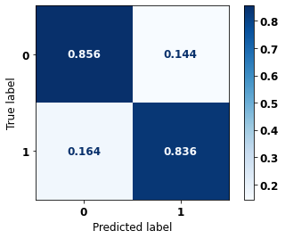
              precision    recall  f1-score   support

           0      0.517     0.856     0.645       264
           1      0.966     0.836     0.896      1287

    accuracy                          0.839      1551
   macro avg      0.742     0.846     0.771      1551
weighted avg      0.890     0.839     0.853      1551
[ ]:
display_confusion_matrix(xgb_fora_00_03, X_testOS_12_15, y_testOS_12_15)

              precision    recall  f1-score   support

           0      0.447     0.856     0.588       292
           1      0.971     0.820     0.889      1715

    accuracy                          0.825      2007
   macro avg      0.709     0.838     0.738      2007
weighted avg      0.895     0.825     0.845      2007
[ ]:
display_confusion_matrix(xgb_fora_00_03, X_testOS_16_20, y_testOS_16_20)
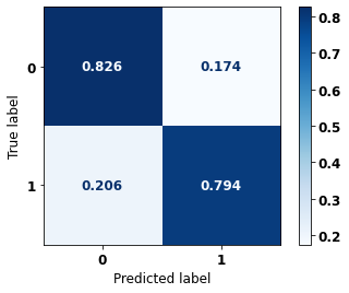
              precision    recall  f1-score   support

           0      0.459     0.826     0.590       304
           1      0.956     0.794     0.867      1438

    accuracy                          0.800      1742
   macro avg      0.707     0.810     0.729      1742
weighted avg      0.869     0.800     0.819      1742
Random Forest Other states for years 2004 to 2007
[ ]:
display_confusion_matrix(rf_fora_04_07, X_testOS_08_11, y_testOS_08_11)
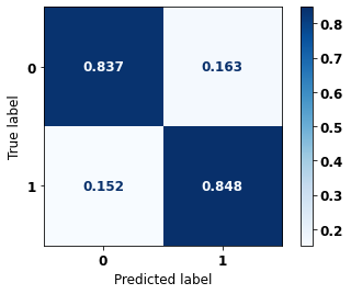
              precision    recall  f1-score   support

           0      0.530     0.837     0.649       264
           1      0.962     0.848     0.901      1287

    accuracy                          0.846      1551
   macro avg      0.746     0.842     0.775      1551
weighted avg      0.889     0.846     0.858      1551
[ ]:
display_confusion_matrix(rf_fora_04_07, X_testOS_12_15, y_testOS_12_15)
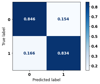
              precision    recall  f1-score   support

           0      0.465     0.846     0.600       292
           1      0.970     0.834     0.897      1715

    accuracy                          0.836      2007
   macro avg      0.717     0.840     0.749      2007
weighted avg      0.896     0.836     0.854      2007
[ ]:
display_confusion_matrix(rf_fora_04_07, X_testOS_16_20, y_testOS_16_20)

              precision    recall  f1-score   support

           0      0.482     0.842     0.613       304
           1      0.960     0.809     0.878      1438

    accuracy                          0.815      1742
   macro avg      0.721     0.825     0.746      1742
weighted avg      0.877     0.815     0.832      1742
XGBoost Other states for years 2004 to 2007
[ ]:
display_confusion_matrix(xgb_fora_04_07, X_testOS_08_11, y_testOS_08_11)

              precision    recall  f1-score   support

           0      0.546     0.848     0.665       264
           1      0.965     0.855     0.907      1287

    accuracy                          0.854      1551
   macro avg      0.756     0.852     0.786      1551
weighted avg      0.894     0.854     0.866      1551
[ ]:
display_confusion_matrix(xgb_fora_04_07, X_testOS_12_15, y_testOS_12_15)

              precision    recall  f1-score   support

           0      0.484     0.856     0.618       292
           1      0.972     0.844     0.904      1715

    accuracy                          0.846      2007
   macro avg      0.728     0.850     0.761      2007
weighted avg      0.901     0.846     0.862      2007
[ ]:
display_confusion_matrix(xgb_fora_04_07, X_testOS_16_20, y_testOS_16_20)

              precision    recall  f1-score   support

           0      0.483     0.836     0.612       304
           1      0.959     0.811     0.879      1438

    accuracy                          0.815      1742
   macro avg      0.721     0.823     0.745      1742
weighted avg      0.876     0.815     0.832      1742
Random Forest Other states for years 2008 to 2011
[ ]:
display_confusion_matrix(rf_fora_08_11, X_testOS_12_15, y_testOS_12_15)
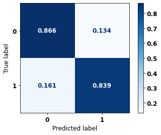
              precision    recall  f1-score   support

           0      0.478     0.866     0.616       292
           1      0.974     0.839     0.901      1715

    accuracy                          0.843      2007
   macro avg      0.726     0.853     0.759      2007
weighted avg      0.902     0.843     0.860      2007
[ ]:
display_confusion_matrix(rf_fora_08_11, X_testOS_16_20, y_testOS_16_20)

              precision    recall  f1-score   support

           0      0.485     0.859     0.620       304
           1      0.964     0.807     0.879      1438

    accuracy                          0.816      1742
   macro avg      0.725     0.833     0.749      1742
weighted avg      0.881     0.816     0.834      1742
XGBoost Other states for years 2008 to 2011
[ ]:
display_confusion_matrix(xgb_fora_08_11, X_testOS_12_15, y_testOS_12_15)

              precision    recall  f1-score   support

           0      0.481     0.856     0.616       292
           1      0.972     0.843     0.903      1715

    accuracy                          0.845      2007
   macro avg      0.726     0.849     0.759      2007
weighted avg      0.900     0.845     0.861      2007
[ ]:
display_confusion_matrix(xgb_fora_08_11, X_testOS_16_20, y_testOS_16_20)

              precision    recall  f1-score   support

           0      0.509     0.845     0.635       304
           1      0.962     0.828     0.890      1438

    accuracy                          0.831      1742
   macro avg      0.735     0.836     0.763      1742
weighted avg      0.883     0.831     0.845      1742
Random Forest Other states for years 2012 to 2015
[ ]:
display_confusion_matrix(rf_fora_12_15, X_testOS_16_20, y_testOS_16_20)

              precision    recall  f1-score   support

           0      0.505     0.829     0.628       304
           1      0.958     0.828     0.888      1438

    accuracy                          0.828      1742
   macro avg      0.732     0.829     0.758      1742
weighted avg      0.879     0.828     0.843      1742
XGBoost Other states for years 2012 to 2015
[ ]:
display_confusion_matrix(xgb_fora_12_15, X_testOS_16_20, y_testOS_16_20)

              precision    recall  f1-score   support

           0      0.503     0.836     0.628       304
           1      0.960     0.825     0.887      1438

    accuracy                          0.827      1742
   macro avg      0.731     0.830     0.758      1742
weighted avg      0.880     0.827     0.842      1742
Fifth approach
Approach with grouped years and without the columns EC and HORMONIO.
Preprocessing
Now we are going to divide the data into training and testing, and then do the preprocessing in both datasets to perform the training of the models and their evaluation. We will use the years grouped too, resulting in 5 datasets for SP and more 5 for other states.
First, it is necessary to define the columns that will be used as features and the label. We will not use some columns of the datasets: UFRESID, because we already have the division between SP and other states in the two datasets.
It was chosen to keep the column IDADE, so we will not use the FAIXAETAR, as well as the column ECGRUP and not the column EC. Finally, the other columns contained in the list list_drop are possible labels, so they will not be used as features for machine learning models.
[ ]:
list_drop = ['UFRESID', 'FAIXAETAR', 'ULTICONS', 'ULTIDIAG', 'ULTITRAT',
             'obito_geral', 'obito_cancer', 'vivo_ano3', 'vivo_ano5',
             'ULTINFO', 'EC', 'HORMONIO']

# 'RECNENHUM', 'RECLOCAL', 'RECREGIO', 'REC01', 'REC02', 'REC03', 'RECDIST'

lb = 'vivo_ano1'
A function was created to perform the preprocessing, preprocessing, that uses the other functions created, get_train_test (divides the dataset into train and test sets), train_preprocessing (do the preprocessing of the train set) and test_preprocessing (do the preprocessing of the test set).
The process will be done 5 times for SP and other states, using the datasets with grouped years.
To see the complete function go to the functions section.
SP
[ ]:
X_trainSP_00_03, X_testSP_00_03, y_trainSP_00_03, y_testSP_00_03, feat_SP_00_03 = preprocessing(df_SP_ano1, list_drop, lb,
                                                                                                group_years=True,
                                                                                                first_year=2000,
                                                                                                last_year=2003,
                                                                                                random_state=seed,
                                                                                                balance_data=False,
                                                                                                encoder_type='LabelEncoder',
                                                                                                norm_name='StandardScaler')
X_train = (47196, 64), X_test = (15732, 64)
y_train = (47196,), y_test = (15732,)
[ ]:
X_trainSP_04_07, X_testSP_04_07, y_trainSP_04_07, y_testSP_04_07, feat_SP_04_07 = preprocessing(df_SP_ano1, list_drop, lb,
                                                                                                group_years=True,
                                                                                                first_year=2004,
                                                                                                last_year=2007,
                                                                                                random_state=seed,
                                                                                                balance_data=False,
                                                                                                encoder_type='LabelEncoder',
                                                                                                norm_name='StandardScaler')
X_train = (59781, 64), X_test = (19928, 64)
y_train = (59781,), y_test = (19928,)
[ ]:
X_trainSP_08_11, X_testSP_08_11, y_trainSP_08_11, y_testSP_08_11, feat_SP_08_11 = preprocessing(df_SP_ano1, list_drop, lb,
                                                                                                group_years=True,
                                                                                                first_year=2008,
                                                                                                last_year=2011,
                                                                                                random_state=seed,
                                                                                                balance_data=False,
                                                                                                encoder_type='LabelEncoder',
                                                                                                norm_name='StandardScaler')
X_train = (80382, 64), X_test = (26795, 64)
y_train = (80382,), y_test = (26795,)
[ ]:
X_trainSP_12_15, X_testSP_12_15, y_trainSP_12_15, y_testSP_12_15, feat_SP_12_15 = preprocessing(df_SP_ano1, list_drop, lb,
                                                                                                group_years=True,
                                                                                                first_year=2012,
                                                                                                last_year=2015,
                                                                                                random_state=seed,
                                                                                                balance_data=False,
                                                                                                encoder_type='LabelEncoder',
                                                                                                norm_name='StandardScaler')
X_train = (99850, 64), X_test = (33284, 64)
y_train = (99850,), y_test = (33284,)
[ ]:
X_trainSP_16_21, X_testSP_16_21, y_trainSP_16_21, y_testSP_16_21, feat_SP_16_21 = preprocessing(df_SP_ano1, list_drop, lb,
                                                                                                group_years=True,
                                                                                                first_year=2016,
                                                                                                last_year=2021,
                                                                                                random_state=seed,
                                                                                                balance_data=False,
                                                                                                encoder_type='LabelEncoder',
                                                                                                norm_name='StandardScaler')
X_train = (65067, 64), X_test = (21689, 64)
y_train = (65067,), y_test = (21689,)
Other states
[ ]:
X_trainOS_00_03, X_testOS_00_03, y_trainOS_00_03, y_testOS_00_03, feat_OS_00_03 = preprocessing(df_fora_ano1, list_drop, lb,
group_years=True,
first_year=2000,
last_year=2003,
random_state=seed,
balance_data=False,
encoder_type='LabelEncoder',
norm_name='StandardScaler')
X_train = (2694, 64), X_test = (899, 64)
y_train = (2694,), y_test = (899,)
[ ]:
X_trainOS_04_07, X_testOS_04_07, y_trainOS_04_07, y_testOS_04_07, feat_OS_04_07 = preprocessing(df_fora_ano1, list_drop, lb,
group_years=True,
first_year=2004,
last_year=2007,
random_state=seed,
balance_data=False,
encoder_type='LabelEncoder',
norm_name='StandardScaler')
X_train = (3738, 64), X_test = (1246, 64)
y_train = (3738,), y_test = (1246,)
[ ]:
X_trainOS_08_11, X_testOS_08_11, y_trainOS_08_11, y_testOS_08_11, feat_OS_08_11 = preprocessing(df_fora_ano1, list_drop, lb,
group_years=True,
first_year=2008,
last_year=2011,
random_state=seed,
balance_data=False,
encoder_type='LabelEncoder',
norm_name='StandardScaler')
X_train = (4652, 64), X_test = (1551, 64)
y_train = (4652,), y_test = (1551,)
[ ]:
X_trainOS_12_15, X_testOS_12_15, y_trainOS_12_15, y_testOS_12_15, feat_OS_12_15 = preprocessing(df_fora_ano1, list_drop, lb,
group_years=True,
first_year=2012,
last_year=2015,
random_state=seed,
balance_data=False,
encoder_type='LabelEncoder',
norm_name='StandardScaler')
X_train = (6019, 64), X_test = (2007, 64)
y_train = (6019,), y_test = (2007,)
[ ]:
X_trainOS_16_20, X_testOS_16_20, y_trainOS_16_20, y_testOS_16_20, feat_OS_16_20 = preprocessing(df_fora_ano1, list_drop, lb,
group_years=True,
first_year=2016,
last_year=2020,
random_state=seed,
balance_data=False,
encoder_type='LabelEncoder',
norm_name='StandardScaler')
X_train = (5223, 64), X_test = (1742, 64)
y_train = (5223,), y_test = (1742,)
Training and evaluation of the models
After dividing the data into training and testing, using the encoder and normalizing, the data is ready to be used by the machine learning models.
Random Forest
The first model is the Random Forest, the random_state will be used as a parameter, to obtain the same training values of the model every time it is runned.
The hyperparameter class_weight was used because the models have difficulty to learn the class with fewer examples.
SP
[ ]:
# SP - 2000 to 2003
rf_sp_00_03 = RandomForestClassifier(random_state=seed,
class_weight={0:3.6, 1:1},
criterion='entropy',
max_depth=10)
rf_sp_00_03.fit(X_trainSP_00_03, y_trainSP_00_03)
RandomForestClassifier(class_weight={0: 3.6, 1: 1}, criterion='entropy',
max_depth=10, random_state=10)
[ ]:
display_confusion_matrix(rf_sp_00_03, X_testSP_00_03, y_testSP_00_03)
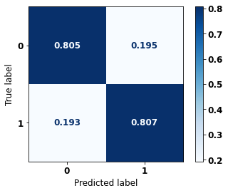
precision recall f1-score support
0 0.538 0.805 0.645 3430
1 0.937 0.807 0.867 12302
accuracy 0.807 15732
macro avg 0.737 0.806 0.756 15732
weighted avg 0.850 0.807 0.819 15732
The confusion matrix obtained for the Random Forest, with SP data from 2000 to 2003, shows a good performance of the model, with 81% of accuracy.
[ ]:
show_tree(rf_sp_00_03, feat_SP_00_03, 2)
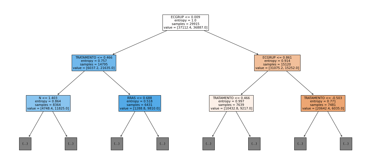
[ ]:
plot_roc_curve(rf_sp_00_03, X_trainSP_00_03, X_testSP_00_03, y_trainSP_00_03, y_testSP_00_03)
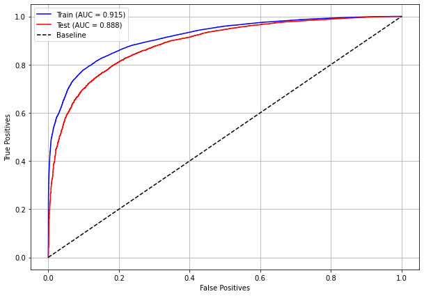
[ ]:
plot_feat_importances(rf_sp_00_03, feat_SP_00_03)
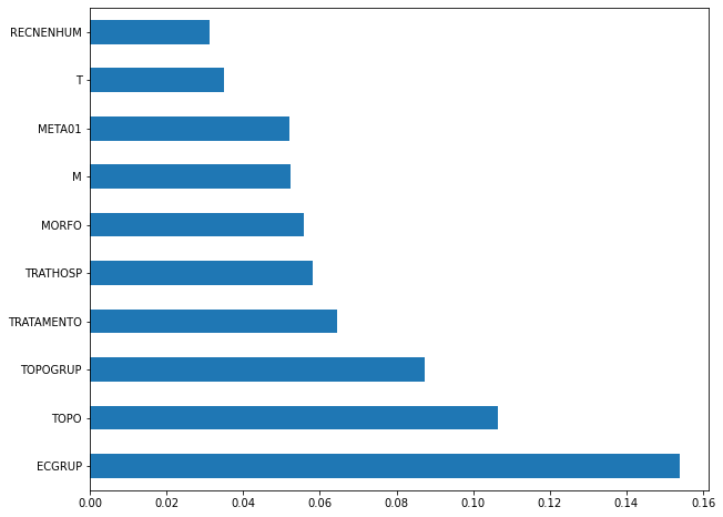
The four most important features in the model were
ECGRUP,TOPO,TOPOGRUP, andTRATAMENTO.
[ ]:
plot_shap_values(rf_sp_00_03, X_testSP_00_03, feat_SP_00_03)
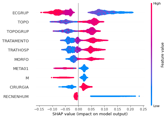
Note that larger values of the ECGRUP column, shown in pink, have more influence for the model’s prediction to be class 0, smaller values have greater weight for the prediction to be class 1. This behavior was expected, because the higher the clinical stage, worse is the stage of cancer.
The other columns shown follow the same logic.
[ ]:
# SP - 2004 to 2007
rf_sp_04_07 = RandomForestClassifier(random_state=seed,
class_weight={0:4.5, 1:1},
criterion='entropy',
max_depth=10)
rf_sp_04_07.fit(X_trainSP_04_07, y_trainSP_04_07)
RandomForestClassifier(class_weight={0: 4.5, 1: 1}, criterion='entropy',
max_depth=10, random_state=10)
[ ]:
display_confusion_matrix(rf_sp_04_07, X_testSP_04_07, y_testSP_04_07)

precision recall f1-score support
0 0.532 0.821 0.646 3955
1 0.949 0.821 0.880 15973
accuracy 0.821 19928
macro avg 0.740 0.821 0.763 19928
weighted avg 0.866 0.821 0.834 19928
The confusion matrix obtained for the Random Forest, with SP data from 2004 to 2007, shows a good performance of the model, with 82% of accuracy.
[ ]:
show_tree(rf_sp_04_07, feat_SP_04_07, 2)
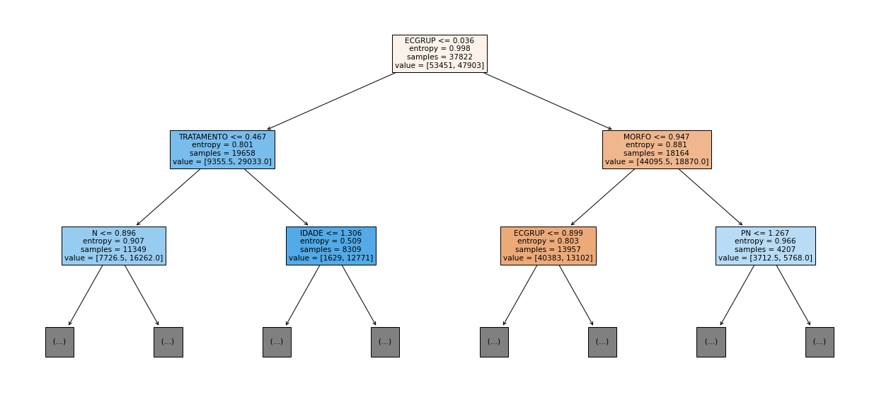
[ ]:
plot_roc_curve(rf_sp_04_07, X_trainSP_04_07, X_testSP_04_07, y_trainSP_04_07, y_testSP_04_07)
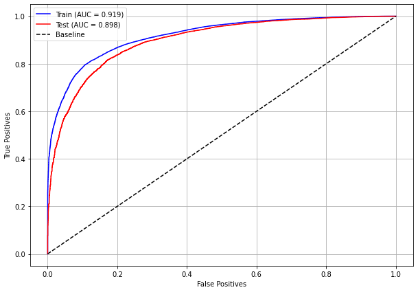
[ ]:
plot_feat_importances(rf_sp_04_07, feat_SP_04_07)
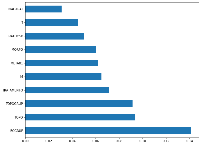
The four most important features in the model were
ECGRUP,TOPO,TOPOGRUPandTRATAMENTO.
[ ]:
plot_shap_values(rf_sp_04_07, X_testSP_04_07, feat_SP_04_07)
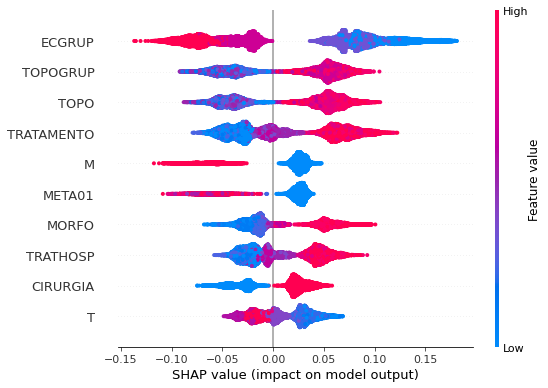
Note that larger values of the ECGRUP column, shown in pink, have more influence for the model’s prediction to be class 0, smaller values have greater weight for the prediction to be class 1. This behavior was expected, because the higher the clinical stage, worse is the stage of cancer.
The other columns shown follow the same logic.
[ ]:
# SP - 2008 to 2011
rf_sp_08_11 = RandomForestClassifier(random_state=seed,
class_weight={0:4.6, 1:1},
criterion='entropy',
max_depth=10)
rf_sp_08_11.fit(X_trainSP_08_11, y_trainSP_08_11)
RandomForestClassifier(class_weight={0: 4.6, 1: 1}, criterion='entropy',
max_depth=10, random_state=10)
[ ]:
display_confusion_matrix(rf_sp_08_11, X_testSP_08_11, y_testSP_08_11)

precision recall f1-score support
0 0.523 0.825 0.640 5020
1 0.954 0.826 0.885 21775
accuracy 0.826 26795
macro avg 0.738 0.826 0.763 26795
weighted avg 0.873 0.826 0.839 26795
The confusion matrix obtained for the Random Forest, with SP data from 2008 to 2011, shows a good performance of the model, with 83% of accuracy.
[ ]:
show_tree(rf_sp_08_11, feat_SP_08_11, 2)
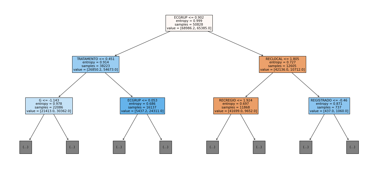
[ ]:
plot_roc_curve(rf_sp_08_11, X_trainSP_08_11, X_testSP_08_11, y_trainSP_08_11, y_testSP_08_11)

[ ]:
plot_feat_importances(rf_sp_08_11, feat_SP_08_11)
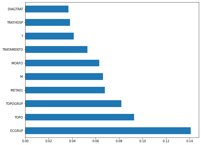
The four most important features in the model were
ECGRUP,TOPO,TOPOGRUPandMETA01.
[ ]:
plot_shap_values(rf_sp_08_11, X_testSP_08_11, feat_SP_08_11)
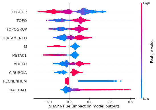
Note that larger values of the ECGRUP column, shown in pink, have more influence for the model’s prediction to be class 0, smaller values have greater weight for the prediction to be class 1. This behavior was expected, because the higher the clinical stage, worse is the stage of cancer.
The other columns shown follow the same logic.
[ ]:
# SP - 2012 to 2015
rf_sp_12_15 = RandomForestClassifier(random_state=seed,
class_weight={0:5.53, 1:1},
criterion='entropy',
max_depth=10)
rf_sp_12_15.fit(X_trainSP_12_15, y_trainSP_12_15)
RandomForestClassifier(class_weight={0: 5.53, 1: 1}, criterion='entropy',
max_depth=10, random_state=10)
[ ]:
display_confusion_matrix(rf_sp_12_15, X_testSP_12_15, y_testSP_12_15)

precision recall f1-score support
0 0.479 0.826 0.607 5442
1 0.960 0.825 0.887 27842
accuracy 0.825 33284
macro avg 0.720 0.825 0.747 33284
weighted avg 0.882 0.825 0.842 33284
The confusion matrix obtained for the Random Forest, with SP data from 2012 to 2015, shows a good performance of the model with 82% of accuracy.
[ ]:
show_tree(rf_sp_12_15, feat_SP_12_15, 2)
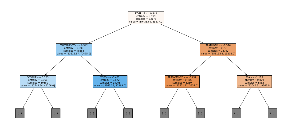
[ ]:
plot_roc_curve(rf_sp_12_15, X_trainSP_12_15, X_testSP_12_15, y_trainSP_12_15, y_testSP_12_15)

[ ]:
plot_feat_importances(rf_sp_12_15, feat_SP_12_15)
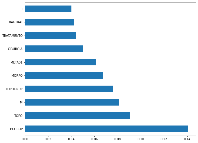
The four most important features in the model were
ECGRUP,TOPO,MandTOPGRUP.
[ ]:
plot_shap_values(rf_sp_12_15, X_testSP_12_15, feat_SP_12_15)
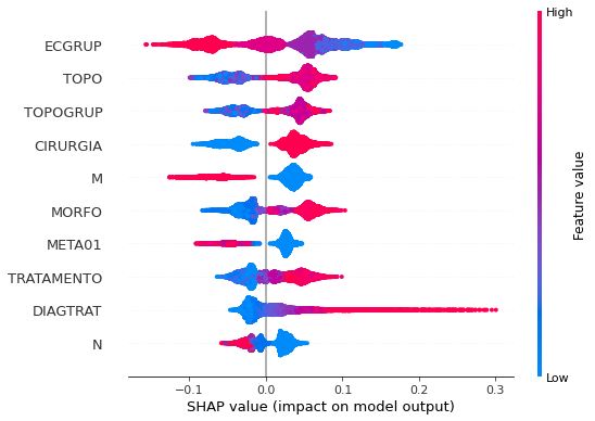
Note that larger values of the ECGRUP column, shown in pink, have more influence for the model’s prediction to be class 0, smaller values have greater weight for the prediction to be class 1. This behavior was expected, because the higher the clinical stage, worse is the stage of cancer.
The other columns shown follow the same logic.
[ ]:
# SP - 2016 to 2021
rf_sp_16_21 = RandomForestClassifier(random_state=seed,
class_weight={0:4.675, 1:1},
criterion='entropy',
max_depth=10)
rf_sp_16_21.fit(X_trainSP_16_21, y_trainSP_16_21)
RandomForestClassifier(class_weight={0: 4.675, 1: 1}, criterion='entropy',
max_depth=10, random_state=10)
[ ]:
display_confusion_matrix(rf_sp_16_21, X_testSP_16_21, y_testSP_16_21)

precision recall f1-score support
0 0.501 0.818 0.621 3944
1 0.953 0.819 0.881 17745
accuracy 0.819 21689
macro avg 0.727 0.818 0.751 21689
weighted avg 0.871 0.819 0.834 21689
The confusion matrix obtained for the Random Forest, with SP data from 2016 to 2021, shows a good performance of the model, with 82% of accuracy.
[ ]:
show_tree(rf_sp_16_21, feat_SP_16_21, 2)
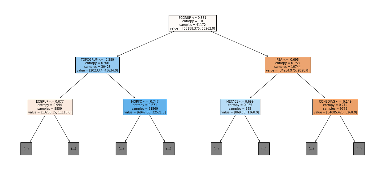
[ ]:
plot_roc_curve(rf_sp_16_21, X_trainSP_16_21, X_testSP_16_21, y_trainSP_16_21, y_testSP_16_21)

[ ]:
plot_feat_importances(rf_sp_16_21, feat_SP_16_21)
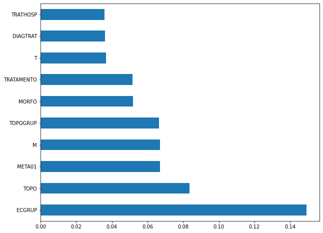
The four most important features in the model were
ECGRUP,TOPO,META01, andM.
[ ]:
plot_shap_values(rf_sp_16_21, X_testSP_16_21, feat_SP_16_21)
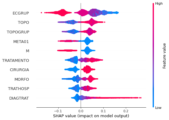
Note that larger values of the ECGRUP column, shown in pink, have more influence for the model’s prediction to be class 0, smaller values have greater weight for the prediction to be class 1. This behavior was expected, because the higher the clinical stage, worse is the stage of cancer.
The other columns shown follow the same logic.
Other states
[ ]:
# Other states - 2000 to 2003
rf_fora_00_03 = RandomForestClassifier(random_state=seed,
class_weight={0:4.735, 1:1},
criterion='entropy',
max_depth=6)
rf_fora_00_03.fit(X_trainOS_00_03, y_trainOS_00_03)
RandomForestClassifier(class_weight={0: 4.735, 1: 1}, criterion='entropy',
max_depth=6, random_state=10)
[ ]:
display_confusion_matrix(rf_fora_00_03, X_testOS_00_03, y_testOS_00_03)
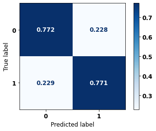
precision recall f1-score support
0 0.457 0.772 0.574 180
1 0.931 0.771 0.843 719
accuracy 0.771 899
macro avg 0.694 0.771 0.709 899
weighted avg 0.836 0.771 0.789 899
The confusion matrix obtained for the Random Forest, with other states data from 2000 to 2003, also shows a good performance of the model, and we have a balanced main diagonal with 77% of accuracy.
[ ]:
show_tree(rf_fora_00_03, feat_OS_00_03, 2)
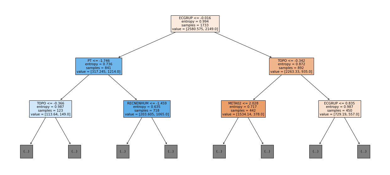
[ ]:
plot_roc_curve(rf_fora_00_03, X_trainOS_00_03, X_testOS_00_03, y_trainOS_00_03, y_testOS_00_03)

[ ]:
plot_feat_importances(rf_fora_00_03, feat_OS_00_03)
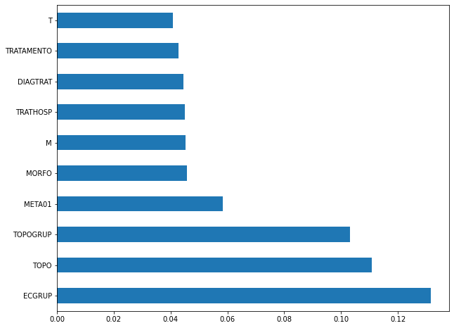
The four most important features in the model were
ECGRUP,TOPO,TOPOGRUPandMETA01.
[ ]:
plot_shap_values(rf_fora_00_03, X_testOS_00_03, feat_OS_00_03)
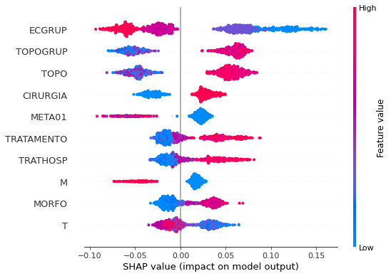
Note that larger values of the ECGRUP column, shown in pink, have more influence for the model’s prediction to be class 0, smaller values have greater weight for the prediction to be class 1. This behavior was expected, because the higher the clinical stage, worse is the stage of cancer.
The other columns shown follow the same logic.
[ ]:
# Other states - 2004 to 2007
rf_fora_04_07 = RandomForestClassifier(random_state=seed,
class_weight={0:4.8, 1:1},
criterion='entropy',
max_depth=6)
rf_fora_04_07.fit(X_trainOS_04_07, y_trainOS_04_07)
RandomForestClassifier(class_weight={0: 4.8, 1: 1}, criterion='entropy',
max_depth=6, random_state=10)
[ ]:
display_confusion_matrix(rf_fora_04_07, X_testOS_04_07, y_testOS_04_07)
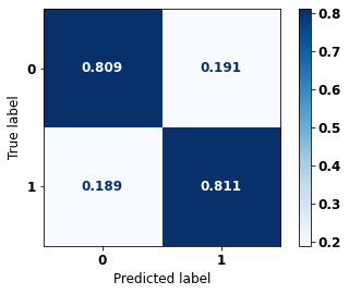
precision recall f1-score support
0 0.485 0.809 0.607 225
1 0.951 0.811 0.875 1021
accuracy 0.811 1246
macro avg 0.718 0.810 0.741 1246
weighted avg 0.867 0.811 0.827 1246
The confusion matrix obtained for the Random Forest, with other states data from 2004 to 2007, also shows a good performance of the model, with 81% of accuracy.
[ ]:
show_tree(rf_fora_04_07, feat_OS_04_07, 2)
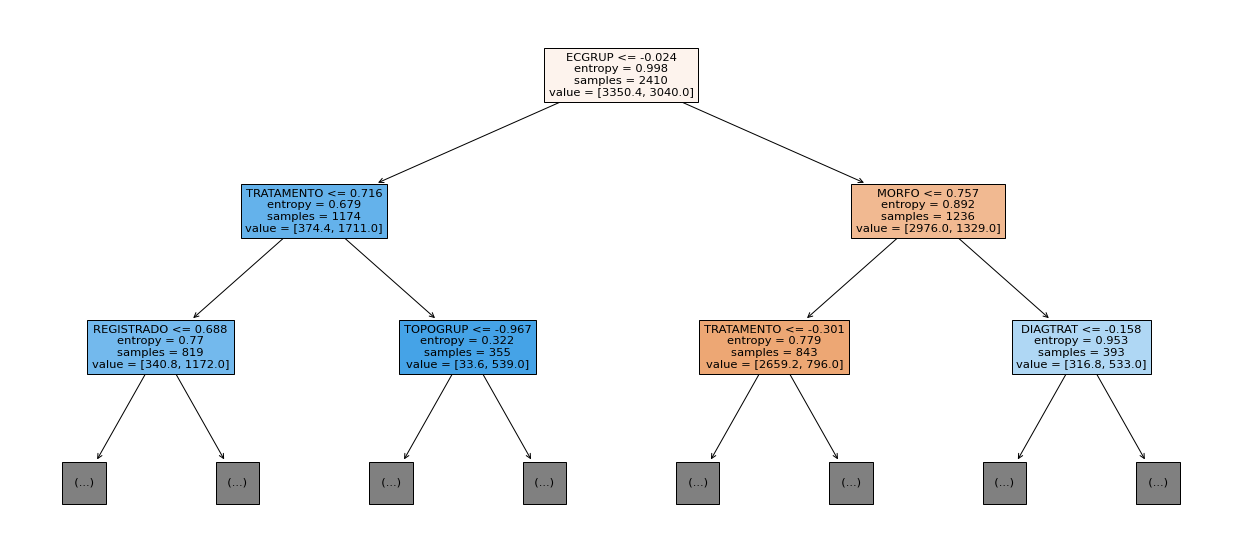
[ ]:
plot_roc_curve(rf_fora_04_07, X_trainOS_04_07, X_testOS_04_07, y_trainOS_04_07, y_testOS_04_07)
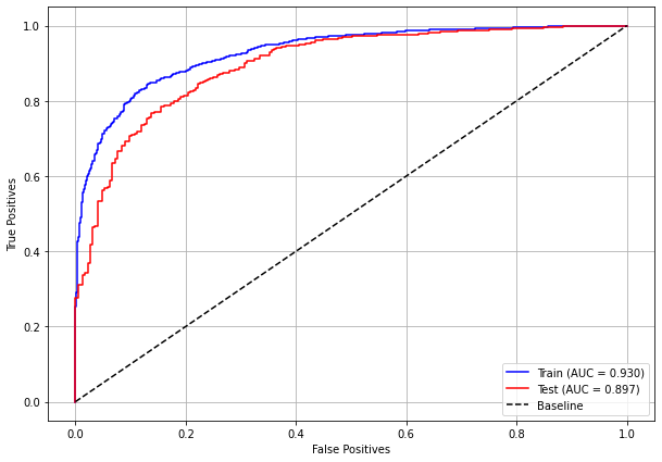
[ ]:
plot_feat_importances(rf_fora_04_07, feat_OS_04_07)
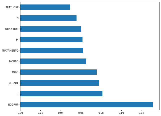
The four most important features in the model were
ECGRUP,T,META01andTOPO.
[ ]:
plot_shap_values(rf_fora_04_07, X_testOS_04_07, feat_OS_04_07)
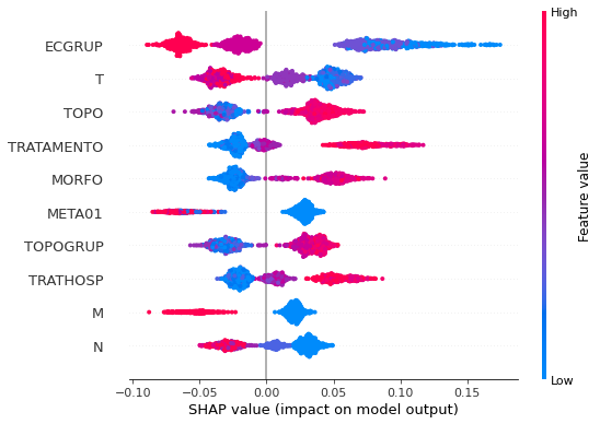
Note that larger values of the ECGRUP column, shown in pink, have more influence for the model’s prediction to be class 0, smaller values have greater weight for the prediction to be class 1. This behavior was expected, because the higher the clinical stage, worse is the stage of cancer.
The other columns shown follow the same logic.
[ ]:
# Other states - 2008 to 2011
rf_fora_08_11 = RandomForestClassifier(random_state=seed,
class_weight={0:7.76, 1:1},
criterion='entropy',
max_depth=7)
rf_fora_08_11.fit(X_trainOS_08_11, y_trainOS_08_11)
RandomForestClassifier(class_weight={0: 7.76, 1: 1}, criterion='entropy',
max_depth=7, random_state=10)
[ ]:
display_confusion_matrix(rf_fora_08_11, X_testOS_08_11, y_testOS_08_11)

precision recall f1-score support
0 0.526 0.845 0.648 264
1 0.964 0.844 0.900 1287
accuracy 0.844 1551
macro avg 0.745 0.844 0.774 1551
weighted avg 0.889 0.844 0.857 1551
The confusion matrix obtained for the Random Forest, with other states data from 2008 to 2011, also shows a good performance of the model, presenting 84% of accuracy.
[ ]:
show_tree(rf_fora_08_11, feat_OS_08_11, 2)
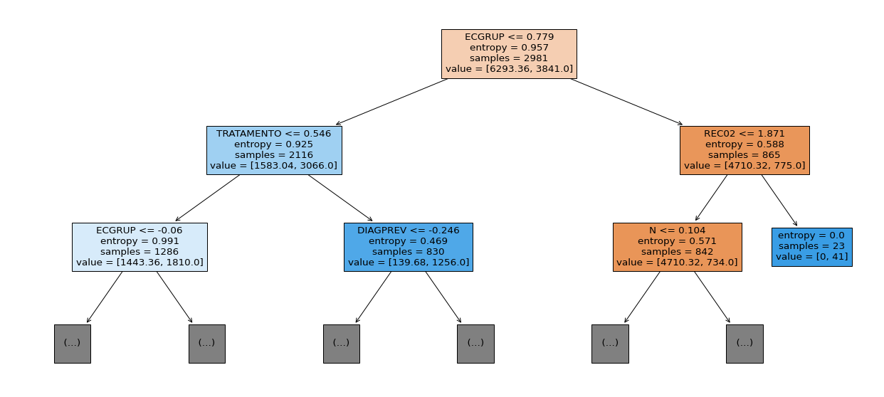
[ ]:
plot_roc_curve(rf_fora_08_11, X_trainOS_08_11, X_testOS_08_11, y_trainOS_08_11, y_testOS_08_11)
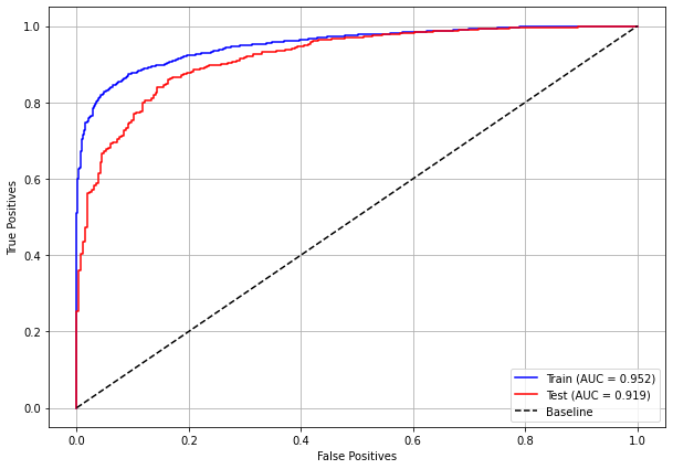
[ ]:
plot_feat_importances(rf_fora_08_11, feat_OS_08_11)
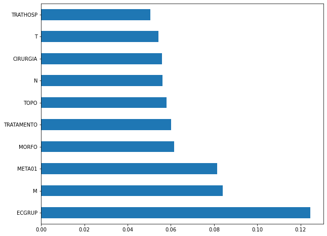
The four most important features in the model were
ECGRUP,M,META01andMORFO.
[ ]:
plot_shap_values(rf_fora_08_11, X_testOS_08_11, feat_OS_08_11)
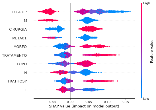
Note that larger values of the ECGRUP column, shown in pink, have more influence for the model’s prediction to be class 0, smaller values have greater weight for the prediction to be class 1. This behavior was expected, because the higher the clinical stage, worse is the stage of cancer.
The other columns shown follow the same logic.
[ ]:
# Other states - 2012 to 2015
rf_fora_12_15 = RandomForestClassifier(random_state=seed,
class_weight={0:6.77, 1:1},
criterion='entropy',
max_depth=7)
rf_fora_12_15.fit(X_trainOS_12_15, y_trainOS_12_15)
RandomForestClassifier(class_weight={0: 6.77, 1: 1}, criterion='entropy',
max_depth=7, random_state=10)
[ ]:
display_confusion_matrix(rf_fora_12_15, X_testOS_12_15, y_testOS_12_15)

precision recall f1-score support
0 0.498 0.853 0.629 292
1 0.971 0.854 0.909 1715
accuracy 0.854 2007
macro avg 0.735 0.853 0.769 2007
weighted avg 0.903 0.854 0.868 2007
The confusion matrix obtained for the Random Forest, with other states data from 2012 to 2015, also shows a good performance of the model, presenting 85% of accuracy.
[ ]:
show_tree(rf_fora_12_15, feat_OS_12_15, 2)
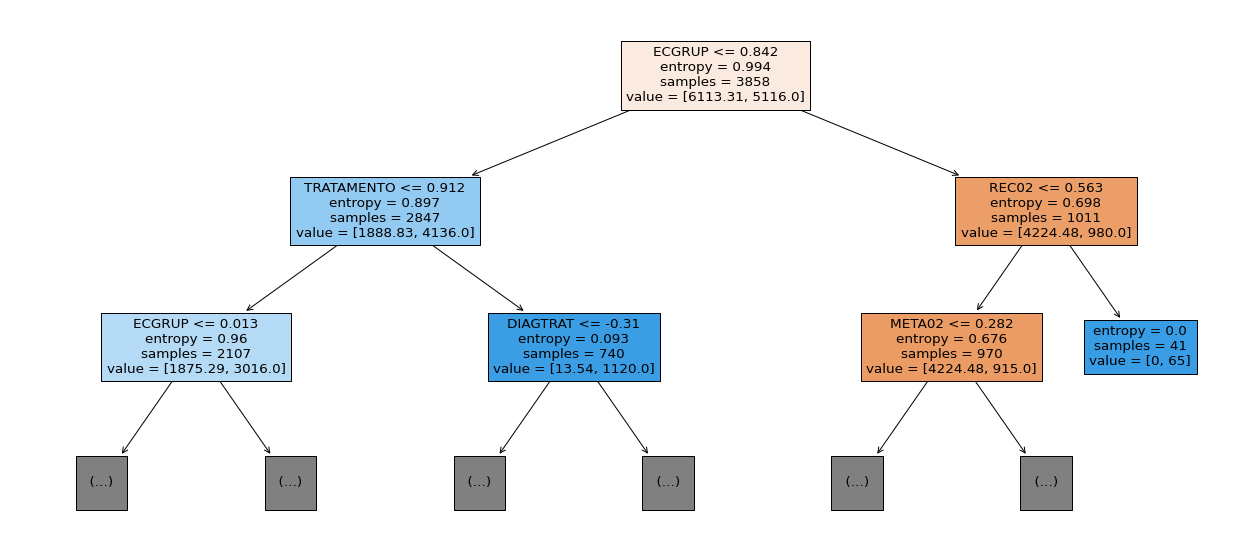
[ ]:
plot_roc_curve(rf_fora_12_15, X_trainOS_12_15, X_testOS_12_15, y_trainOS_12_15, y_testOS_12_15)
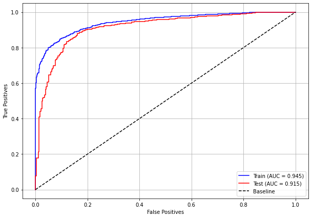
[ ]:
plot_feat_importances(rf_fora_12_15, feat_OS_12_15)
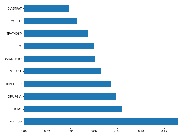
The four most important features in the model were
ECGRUP,TOPO,CIRURGIAandTOPOGRUP.
[ ]:
plot_shap_values(rf_fora_12_15, X_testOS_12_15, feat_OS_12_15)
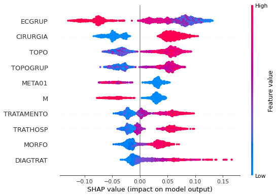
Note that larger values of the ECGRUP column, shown in pink, have more influence for the model’s prediction to be class 0, smaller values have greater weight for the prediction to be class 1. This behavior was expected, because the higher the clinical stage, worse is the stage of cancer.
The other columns shown follow the same logic.
[ ]:
# Other states - 2016 to 2020
rf_fora_16_20 = RandomForestClassifier(random_state=seed,
class_weight={0:4.8, 1:1},
criterion='entropy',
max_depth=7)
rf_fora_16_20.fit(X_trainOS_16_20, y_trainOS_16_20)
RandomForestClassifier(class_weight={0: 4.8, 1: 1}, criterion='entropy',
max_depth=7, random_state=10)
[ ]:
display_confusion_matrix(rf_fora_16_20, X_testOS_16_20, y_testOS_16_20)

precision recall f1-score support
0 0.524 0.839 0.645 304
1 0.961 0.839 0.896 1438
accuracy 0.839 1742
macro avg 0.742 0.839 0.770 1742
weighted avg 0.885 0.839 0.852 1742
The confusion matrix obtained for the Random Forest, with other states data from 2016 to 2020, also shows a good performance of the model, presenting 84% of accuracy.
[ ]:
show_tree(rf_fora_16_20, feat_OS_16_20, 2)
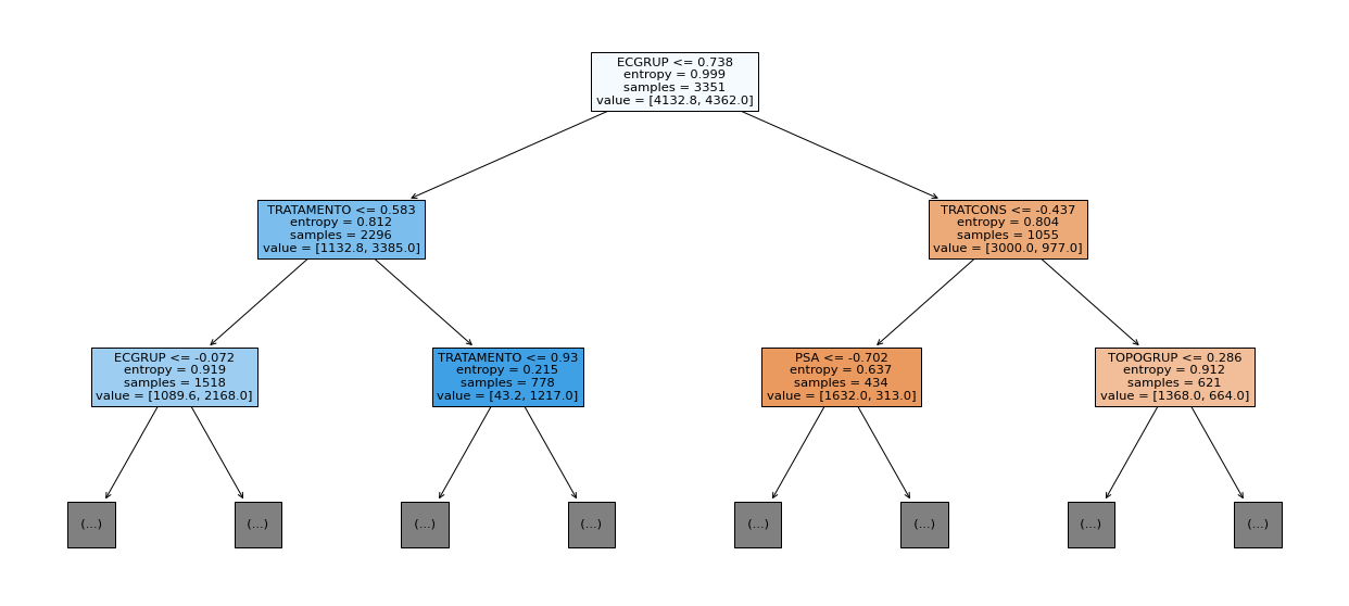
[ ]:
plot_roc_curve(rf_fora_16_20, X_trainOS_16_20, X_testOS_16_20, y_trainOS_16_20, y_testOS_16_20)

[ ]:
plot_feat_importances(rf_fora_16_20, feat_OS_16_20)
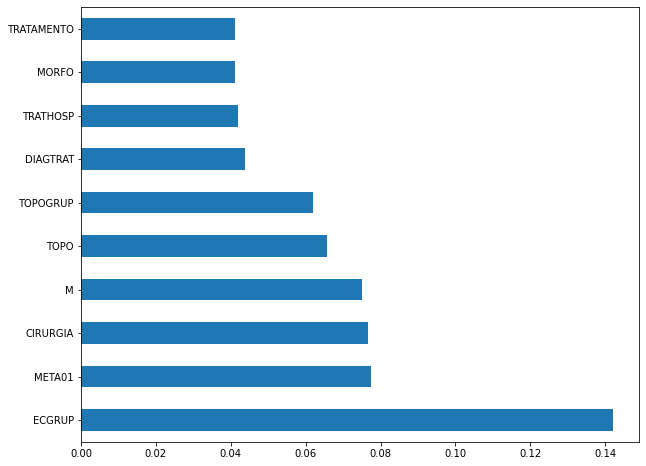
The four most important features in the model were
ECGRUP,META01,CIRURGIAandM.
[ ]:
plot_shap_values(rf_fora_16_20, X_testOS_16_20, feat_OS_16_20)
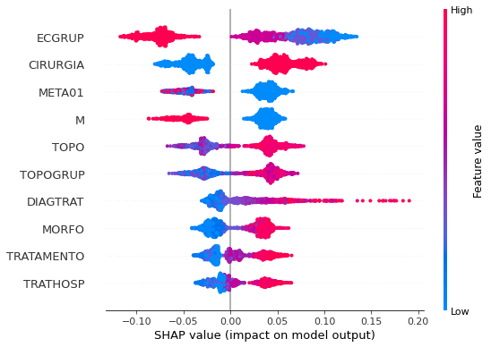
Note that larger values of the ECGRUP column, shown in pink, have more influence for the model’s prediction to be class 0, smaller values have greater weight for the prediction to be class 1. This behavior was expected, because the higher the clinical stage, worse is the stage of cancer.
The other columns shown follow the same logic.
XGBoost
The training of the XGBoost models follows the same pattern with random_state. The hyperparameter scale_pos_weight was also used in the trainings, in order to obtain a balanced main diagonal in the confusion matrix.
The hyperparameter max_depth was chosen as 10 because the default value for this hyperparameter is 3, a low value for the amount of data we have.
SP
[ ]:
# SP - 2000 to 2003
xgb_sp_00_03 = XGBClassifier(max_depth=8,
random_state=seed,
scale_pos_weight=0.27)
xgb_sp_00_03.fit(X_trainSP_00_03, y_trainSP_00_03)
XGBClassifier(max_depth=8, random_state=10, scale_pos_weight=0.27)
[ ]:
display_confusion_matrix(xgb_sp_00_03, X_testSP_00_03, y_testSP_00_03)

precision recall f1-score support
0 0.562 0.821 0.668 3430
1 0.943 0.822 0.878 12302
accuracy 0.822 15732
macro avg 0.753 0.822 0.773 15732
weighted avg 0.860 0.822 0.832 15732
The confusion matrix obtained for the XGBoost, with SP data from 2000 to 2003, shows a good performance of the model, here with 82% of accuracy.
[ ]:
plot_roc_curve(xgb_sp_00_03, X_trainSP_00_03, X_testSP_00_03, y_trainSP_00_03, y_testSP_00_03)
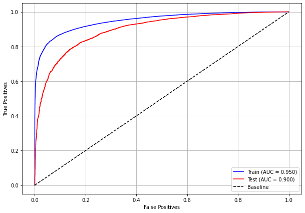
[ ]:
plot_feat_importances(xgb_sp_00_03, feat_SP_00_03)
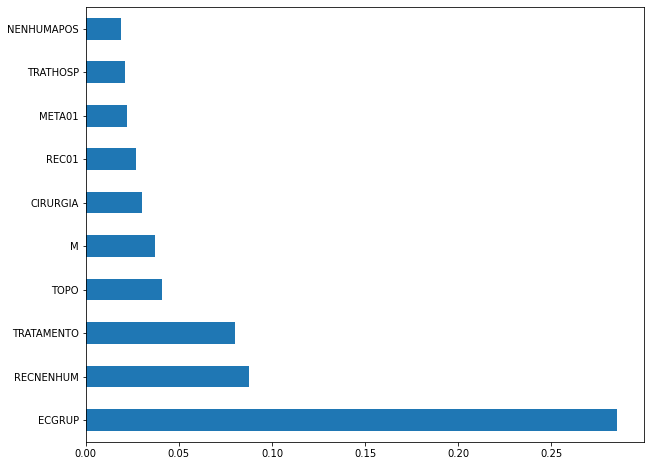
Here we noticed that the most used feature was
ECGRUP, with a lot advantage over the others. Following we haveRECNENHUM,TRATAMENTOandTOPO.
[ ]:
plot_shap_values(xgb_sp_00_03, X_testSP_00_03, feat_SP_00_03)
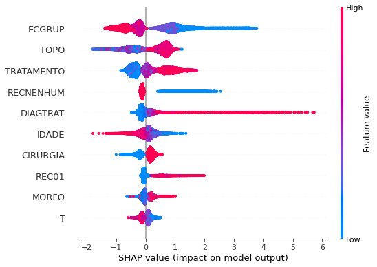
Note that larger values of the ECGRUP column, shown in pink, have more influence for the model’s prediction to be class 0, smaller values have greater weight for the prediction to be class 1. This behavior was expected, because the higher the clinical stage, worse is the stage of cancer.
The other columns shown follow the same logic.
[ ]:
# SP - 2004 to 2007
xgb_sp_04_07 = XGBClassifier(max_depth=8,
random_state=seed,
scale_pos_weight=0.22)
xgb_sp_04_07.fit(X_trainSP_04_07, y_trainSP_04_07)
XGBClassifier(max_depth=8, random_state=10, scale_pos_weight=0.22)
[ ]:
display_confusion_matrix(xgb_sp_04_07, X_testSP_04_07, y_testSP_04_07)

precision recall f1-score support
0 0.546 0.830 0.659 3955
1 0.952 0.829 0.886 15973
accuracy 0.829 19928
macro avg 0.749 0.829 0.772 19928
weighted avg 0.871 0.829 0.841 19928
The confusion matrix obtained for the XGBoost, with SP data from 2004 to 2007, shows a good performance of the model, with 83% of accuracy.
[ ]:
plot_roc_curve(xgb_sp_04_07, X_trainSP_04_07, X_testSP_04_07, y_trainSP_04_07, y_testSP_04_07)

[ ]:
plot_feat_importances(xgb_sp_04_07, feat_SP_04_07)
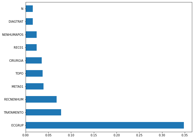
Here we noticed that the most used feature was
ECGRUP, with a good advantage over the others. Following we haveTRATAMENTO,RECNENHUMandMETA01.
[ ]:
plot_shap_values(xgb_sp_04_07, X_testSP_04_07, feat_SP_04_07)
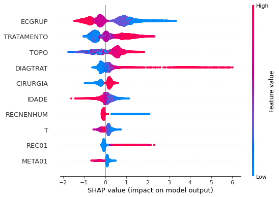
Note that larger values of the ECGRUP column, shown in pink, have more influence for the model’s prediction to be class 0, smaller values have greater weight for the prediction to be class 1. This behavior was expected, because the higher the clinical stage, worse is the stage of cancer.
The other columns shown follow the same logic.
[ ]:
# SP - 2008 to 2011
xgb_sp_08_11 = XGBClassifier(max_depth=8,
scale_pos_weight=0.217,
random_state=seed)
xgb_sp_08_11.fit(X_trainSP_08_11, y_trainSP_08_11)
XGBClassifier(max_depth=8, random_state=10, scale_pos_weight=0.217)
[ ]:
display_confusion_matrix(xgb_sp_08_11, X_testSP_08_11, y_testSP_08_11)

precision recall f1-score support
0 0.552 0.842 0.667 5020
1 0.959 0.843 0.897 21775
accuracy 0.842 26795
macro avg 0.755 0.842 0.782 26795
weighted avg 0.882 0.842 0.854 26795
The confusion matrix obtained for the XGBoost, with SP data from 2008 to 2011, shows a good performance of the model, with 84% of accuracy.
[ ]:
plot_roc_curve(xgb_sp_08_11, X_trainSP_08_11, X_testSP_08_11, y_trainSP_08_11, y_testSP_08_11)

[ ]:
plot_feat_importances(xgb_sp_08_11, feat_SP_08_11)
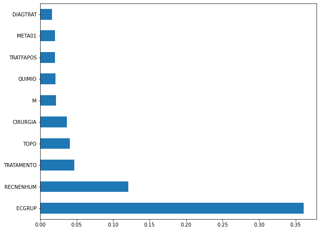
Here we noticed that the most used feature was
ECGRUP, with a good advantage over the others. Following we haveRECNENHUM,TRATAMENTOandTOPO.
[ ]:
plot_shap_values(xgb_sp_08_11, X_testSP_08_11, feat_SP_08_11)
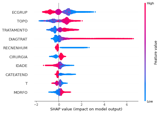
Note that larger values of the ECGRUP column, shown in pink, have more influence for the model’s prediction to be class 0, smaller values have greater weight for the prediction to be class 1. This behavior was expected, because the higher the clinical stage, worse is the stage of cancer.
The other columns shown follow the same logic.
[ ]:
# SP - 2012 to 2015
xgb_sp_12_15 = XGBClassifier(max_depth=8,
random_state=seed,
scale_pos_weight=0.185)
xgb_sp_12_15.fit(X_trainSP_12_15, y_trainSP_12_15)
XGBClassifier(max_depth=8, random_state=10, scale_pos_weight=0.185)
[ ]:
display_confusion_matrix(xgb_sp_12_15, X_testSP_12_15, y_testSP_12_15)

precision recall f1-score support
0 0.505 0.840 0.631 5442
1 0.964 0.839 0.897 27842
accuracy 0.839 33284
macro avg 0.735 0.840 0.764 33284
weighted avg 0.889 0.839 0.854 33284
The confusion matrix obtained for the XGBoost, with SP data from 2012 to 2015, shows a good performance of the model, with 84% of accuracy.
[ ]:
plot_roc_curve(xgb_sp_12_15, X_trainSP_12_15, X_testSP_12_15, y_trainSP_12_15, y_testSP_12_15)
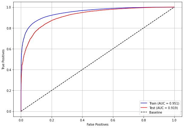
[ ]:
plot_feat_importances(xgb_sp_12_15, feat_SP_12_15)
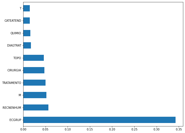
Here we noticed that the most used feature was
ECGRUP, with a good advantage. Following we haveRECNENHUM,MandTRATAMENTO.
[ ]:
plot_shap_values(xgb_sp_12_15, X_testSP_12_15, feat_SP_12_15)
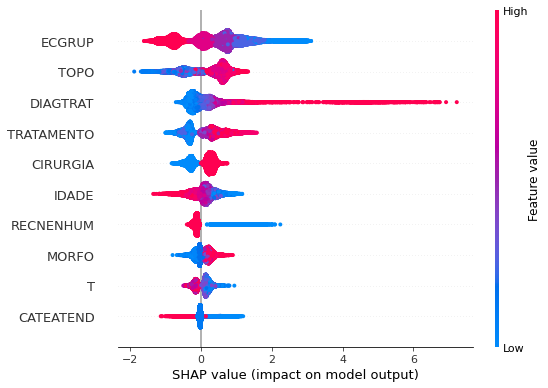
Note that larger values of the ECGRUP column, shown in pink, have more influence for the model’s prediction to be class 0, smaller values have greater weight for the prediction to be class 1. This behavior was expected, because the higher the clinical stage, worse is the stage of cancer.
The other columns shown follow the same logic.
[ ]:
# SP - 2016 to 2021
xgb_sp_16_21 = XGBClassifier(max_depth=8,
random_state=seed,
scale_pos_weight=0.206)
xgb_sp_16_21.fit(X_trainSP_16_21, y_trainSP_16_21)
XGBClassifier(max_depth=8, random_state=10, scale_pos_weight=0.206)
[ ]:
display_confusion_matrix(xgb_sp_16_21, X_testSP_16_21, y_testSP_16_21)

precision recall f1-score support
0 0.525 0.833 0.644 3944
1 0.957 0.832 0.890 17745
accuracy 0.832 21689
macro avg 0.741 0.833 0.767 21689
weighted avg 0.879 0.832 0.846 21689
The confusion matrix obtained for the XGBoost, with SP data from 2016 to 2021, shows a good performance of the model, with 83% of accuracy.
[ ]:
plot_roc_curve(xgb_sp_16_21, X_trainSP_16_21, X_testSP_16_21, y_trainSP_16_21, y_testSP_16_21)
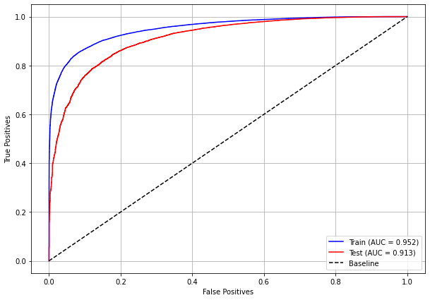
[ ]:
plot_feat_importances(xgb_sp_16_21, feat_SP_16_21)
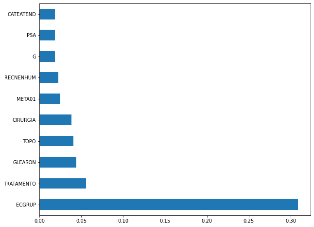
The four most important features were
ECGRUP,TRATAMENTO,GLEASONandTOPO.
[ ]:
plot_shap_values(xgb_sp_16_21, X_testSP_16_21, feat_SP_16_21)
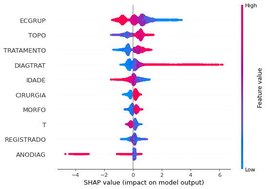
Note that larger values of the ECGRUP column, shown in pink, have more influence for the model’s prediction to be class 0, smaller values have greater weight for the prediction to be class 1. This behavior was expected, because the higher the clinical stage, worse is the stage of cancer.
The other columns shown follow the same logic.
Other states
[ ]:
# Other states - 2000 to 2003
xgb_fora_00_03 = XGBClassifier(max_depth=4,
scale_pos_weight=0.2083,
random_state=seed)
xgb_fora_00_03.fit(X_trainOS_00_03, y_trainOS_00_03)
XGBClassifier(max_depth=4, random_state=10, scale_pos_weight=0.2083)
[ ]:
display_confusion_matrix(xgb_fora_00_03, X_testOS_00_03, y_testOS_00_03)
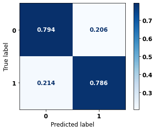
precision recall f1-score support
0 0.481 0.794 0.600 180
1 0.939 0.786 0.855 719
accuracy 0.788 899
macro avg 0.710 0.790 0.727 899
weighted avg 0.847 0.788 0.804 899
The confusion matrix obtained for the XGBoost, with other states data from 2000 to 2003, also shows a good performance of the model, with 79% of accuracy.
[ ]:
plot_roc_curve(xgb_fora_00_03, X_trainOS_00_03, X_testOS_00_03, y_trainOS_00_03, y_testOS_00_03)
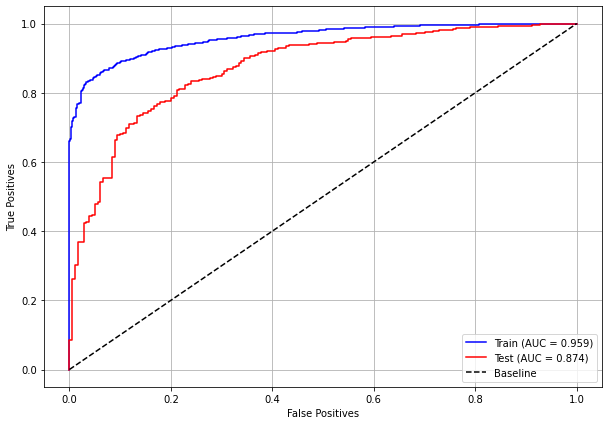
[ ]:
plot_feat_importances(xgb_fora_00_03, feat_OS_00_03)
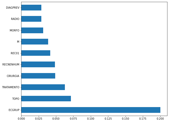
Again we noticed that the most used feature was
ECGRUP, with a good advantage. The following most important features wereTOPO,TRATAMENTOandCIRURGIA.
[ ]:
plot_shap_values(xgb_fora_00_03, X_testOS_00_03, feat_OS_00_03)
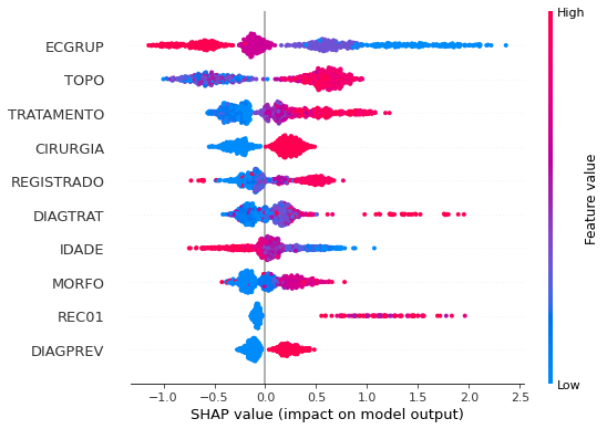
Note that larger values of the ECGRUP column, shown in pink, have more influence for the model’s prediction to be class 0, smaller values have greater weight for the prediction to be class 1. This behavior was expected, because the higher the clinical stage, worse is the stage of cancer.
The other columns shown follow the same logic.
[ ]:
# Other states - 2004 to 2007
xgb_fora_04_07 = XGBClassifier(max_depth=4,
scale_pos_weight=0.22,
random_state=seed)
xgb_fora_04_07.fit(X_trainOS_04_07, y_trainOS_04_07)
XGBClassifier(max_depth=4, random_state=10, scale_pos_weight=0.22)
[ ]:
display_confusion_matrix(xgb_fora_04_07, X_testOS_04_07, y_testOS_04_07)
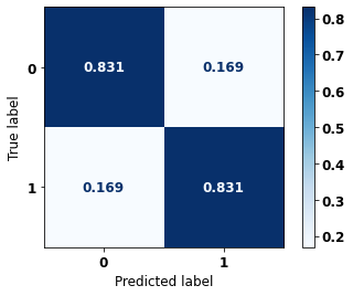
precision recall f1-score support
0 0.519 0.831 0.639 225
1 0.957 0.831 0.889 1021
accuracy 0.831 1246
macro avg 0.738 0.831 0.764 1246
weighted avg 0.878 0.831 0.844 1246
The confusion matrix obtained for the XGBoost, with other states data from 2004 to 2007, also shows a good performance of the model with 83% of accuracy.
[ ]:
plot_roc_curve(xgb_fora_04_07, X_trainOS_04_07, X_testOS_04_07, y_trainOS_04_07, y_testOS_04_07)
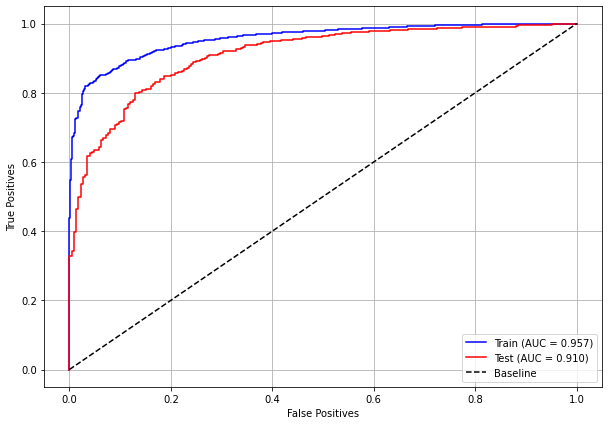
[ ]:
plot_feat_importances(xgb_fora_04_07, feat_OS_04_07)
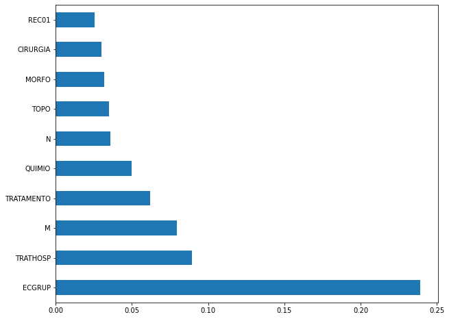
Again we noticed that the most used feature was
ECGRUP, with a good advantage. The following most important features wereTRATHOSP,MandTRATAMENTO.
[ ]:
plot_shap_values(xgb_fora_04_07, X_testOS_04_07, feat_OS_04_07)
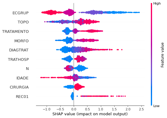
Note that larger values of the ECGRUP column, shown in pink, have more influence for the model’s prediction to be class 0, smaller values have greater weight for the prediction to be class 1. This behavior was expected, because the higher the clinical stage, worse is the stage of cancer.
The other columns shown follow the same logic.
[ ]:
# Other states - 2008 to 2011
xgb_fora_08_11 = XGBClassifier(max_depth=5,
scale_pos_weight=0.145,
random_state=seed)
xgb_fora_08_11.fit(X_trainOS_08_11, y_trainOS_08_11)
XGBClassifier(max_depth=5, random_state=10, scale_pos_weight=0.145)
[ ]:
display_confusion_matrix(xgb_fora_08_11, X_testOS_08_11, y_testOS_08_11)

precision recall f1-score support
0 0.540 0.852 0.661 264
1 0.966 0.851 0.905 1287
accuracy 0.851 1551
macro avg 0.753 0.852 0.783 1551
weighted avg 0.893 0.851 0.863 1551
The confusion matrix obtained for the XGBoost, with other states data from 2008 to 2011, also shows a good performance of the model with 85% of accuracy.
[ ]:
plot_roc_curve(xgb_fora_08_11, X_trainOS_08_11, X_testOS_08_11, y_trainOS_08_11, y_testOS_08_11)

[ ]:
plot_feat_importances(xgb_fora_08_11, feat_OS_08_11)
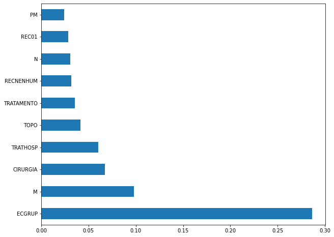
Again we noticed that the most used feature was
ECGRUP, but not with a lot of advantage. The following most important features wereM,CIRURGIAandTRATHOSP.
[ ]:
plot_shap_values(xgb_fora_08_11, X_testOS_08_11, feat_OS_08_11)
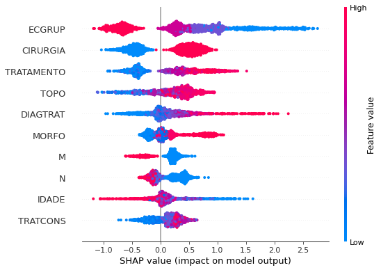
Note that larger values of the ECGRUP column, shown in pink, have more influence for the model’s prediction to be class 0, smaller values have greater weight for the prediction to be class 1. This behavior was expected, because the higher the clinical stage, worse is the stage of cancer.
The other columns shown follow the same logic.
[ ]:
# Other states - 2012 to 2015
xgb_fora_12_15 = XGBClassifier(max_depth=5,
scale_pos_weight=0.1415,
random_state=seed)
xgb_fora_12_15.fit(X_trainOS_12_15, y_trainOS_12_15)
XGBClassifier(max_depth=5, random_state=10, scale_pos_weight=0.1415)
[ ]:
display_confusion_matrix(xgb_fora_12_15, X_testOS_12_15, y_testOS_12_15)

precision recall f1-score support
0 0.498 0.853 0.629 292
1 0.971 0.854 0.909 1715
accuracy 0.854 2007
macro avg 0.735 0.853 0.769 2007
weighted avg 0.903 0.854 0.868 2007
The confusion matrix obtained for the XGBoost, with other states data from 2012 to 2015, also shows a good performance of the model with 85% of accuracy.
[ ]:
plot_roc_curve(xgb_fora_12_15, X_trainOS_12_15, X_testOS_12_15, y_trainOS_12_15, y_testOS_12_15)

[ ]:
plot_feat_importances(xgb_fora_12_15, feat_OS_12_15)
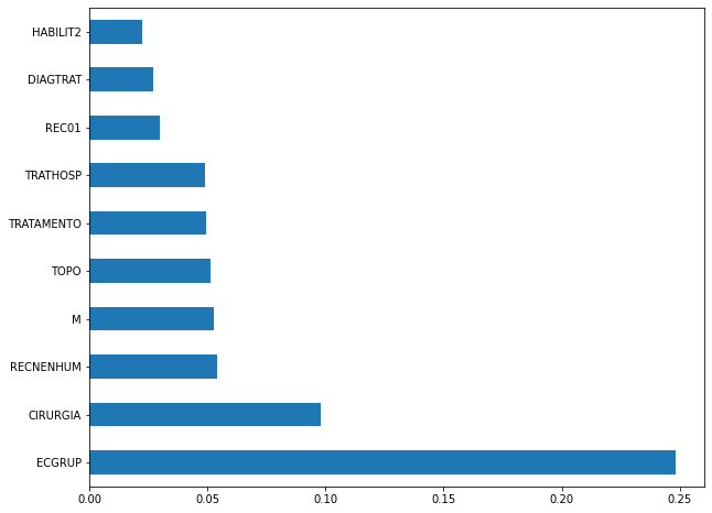
The four most important features were
ECGRUP,CIRURGIA,RECNENHUMandM.
[ ]:
plot_shap_values(xgb_fora_12_15, X_testOS_12_15, feat_OS_12_15)
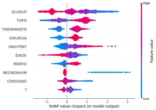
Note that larger values of the ECGRUP column, shown in pink, have more influence for the model’s prediction to be class 0, smaller values have greater weight for the prediction to be class 1. This behavior was expected, because the higher the clinical stage, worse is the stage of cancer.
The other columns shown follow the same logic.
[ ]:
# Other states - 2016 to 2020
xgb_fora_16_20 = XGBClassifier(max_depth=5,
scale_pos_weight=0.164,
random_state=seed)
xgb_fora_16_20.fit(X_trainOS_16_20, y_trainOS_16_20)
XGBClassifier(max_depth=5, random_state=10, scale_pos_weight=0.164)
[ ]:
display_confusion_matrix(xgb_fora_16_20, X_testOS_16_20, y_testOS_16_20)

precision recall f1-score support
0 0.518 0.836 0.640 304
1 0.960 0.836 0.894 1438
accuracy 0.836 1742
macro avg 0.739 0.836 0.767 1742
weighted avg 0.883 0.836 0.849 1742
The confusion matrix obtained for the XGBoost, with other states data from 2016 to 2020, shows the best performance comparing with the other models, with 84% of accuracy.
[ ]:
plot_roc_curve(xgb_fora_16_20, X_trainOS_16_20, X_testOS_16_20, y_trainOS_16_20, y_testOS_16_20)

[ ]:
plot_feat_importances(xgb_fora_16_20, feat_OS_16_20)
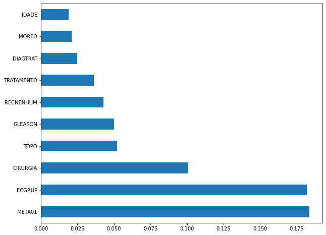
The four most important features were
ECGRUP,META01,CIRURGIAandTOPO.
[ ]:
plot_shap_values(xgb_fora_16_20, X_testOS_16_20, feat_OS_16_20)
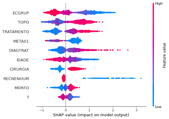
Note that larger values of the ECGRUP column, shown in pink, have more influence for the model’s prediction to be class 0, smaller values have greater weight for the prediction to be class 1. This behavior was expected, because the higher the clinical stage, worse is the stage of cancer.
The other columns shown follow the same logic.
Testing models with data from other years
We will use test data from the following years in the trained models for each set of years grouped together.
Random Forest SP for years 2000 to 2003
[ ]:
display_confusion_matrix(rf_sp_00_03, X_testSP_04_07, y_testSP_04_07)

precision recall f1-score support
0 0.538 0.796 0.642 3955
1 0.943 0.830 0.883 15973
accuracy 0.824 19928
macro avg 0.740 0.813 0.762 19928
weighted avg 0.862 0.824 0.835 19928
[ ]:
display_confusion_matrix(rf_sp_00_03, X_testSP_08_11, y_testSP_08_11)

precision recall f1-score support
0 0.544 0.772 0.638 5020
1 0.942 0.851 0.894 21775
accuracy 0.836 26795
macro avg 0.743 0.811 0.766 26795
weighted avg 0.867 0.836 0.846 26795
[ ]:
display_confusion_matrix(rf_sp_00_03, X_testSP_12_15, y_testSP_12_15)

precision recall f1-score support
0 0.494 0.743 0.594 5442
1 0.944 0.851 0.895 27842
accuracy 0.834 33284
macro avg 0.719 0.797 0.745 33284
weighted avg 0.871 0.834 0.846 33284
[ ]:
display_confusion_matrix(rf_sp_00_03, X_testSP_16_21, y_testSP_16_21)

precision recall f1-score support
0 0.503 0.708 0.588 3944
1 0.929 0.844 0.884 17745
accuracy 0.819 21689
macro avg 0.716 0.776 0.736 21689
weighted avg 0.851 0.819 0.830 21689
XGBoost SP for years 2000 to 2003
[ ]:
display_confusion_matrix(xgb_sp_00_03, X_testSP_04_07, y_testSP_04_07)

precision recall f1-score support
0 0.574 0.753 0.651 3955
1 0.934 0.861 0.896 15973
accuracy 0.840 19928
macro avg 0.754 0.807 0.774 19928
weighted avg 0.862 0.840 0.848 19928
[ ]:
display_confusion_matrix(xgb_sp_00_03, X_testSP_08_11, y_testSP_08_11)

precision recall f1-score support
0 0.580 0.740 0.650 5020
1 0.936 0.877 0.905 21775
accuracy 0.851 26795
macro avg 0.758 0.808 0.778 26795
weighted avg 0.869 0.851 0.858 26795
[ ]:
display_confusion_matrix(xgb_sp_00_03, X_testSP_12_15, y_testSP_12_15)

precision recall f1-score support
0 0.506 0.729 0.597 5442
1 0.942 0.861 0.900 27842
accuracy 0.839 33284
macro avg 0.724 0.795 0.749 33284
weighted avg 0.871 0.839 0.850 33284
[ ]:
display_confusion_matrix(xgb_sp_00_03, X_testSP_16_21, y_testSP_16_21)

precision recall f1-score support
0 0.509 0.705 0.591 3944
1 0.928 0.849 0.887 17745
accuracy 0.822 21689
macro avg 0.718 0.777 0.739 21689
weighted avg 0.852 0.822 0.833 21689
Random Forest SP for years 2004 to 2007
[ ]:
display_confusion_matrix(rf_sp_04_07, X_testSP_08_11, y_testSP_08_11)

precision recall f1-score support
0 0.525 0.798 0.633 5020
1 0.947 0.833 0.887 21775
accuracy 0.827 26795
macro avg 0.736 0.815 0.760 26795
weighted avg 0.868 0.827 0.839 26795
[ ]:
display_confusion_matrix(rf_sp_04_07, X_testSP_12_15, y_testSP_12_15)

precision recall f1-score support
0 0.484 0.771 0.595 5442
1 0.949 0.839 0.891 27842
accuracy 0.828 33284
macro avg 0.717 0.805 0.743 33284
weighted avg 0.873 0.828 0.842 33284
[ ]:
display_confusion_matrix(rf_sp_04_07, X_testSP_16_21, y_testSP_16_21)

precision recall f1-score support
0 0.504 0.724 0.594 3944
1 0.932 0.842 0.885 17745
accuracy 0.820 21689
macro avg 0.718 0.783 0.739 21689
weighted avg 0.854 0.820 0.832 21689
XGBoost SP for years 2004 to 2007
[ ]:
display_confusion_matrix(xgb_sp_04_07, X_testSP_08_11, y_testSP_08_11)

precision recall f1-score support
0 0.552 0.798 0.653 5020
1 0.948 0.851 0.897 21775
accuracy 0.841 26795
macro avg 0.750 0.825 0.775 26795
weighted avg 0.874 0.841 0.851 26795
[ ]:
display_confusion_matrix(xgb_sp_04_07, X_testSP_12_15, y_testSP_12_15)

precision recall f1-score support
0 0.497 0.758 0.601 5442
1 0.947 0.850 0.896 27842
accuracy 0.835 33284
macro avg 0.722 0.804 0.748 33284
weighted avg 0.874 0.835 0.848 33284
[ ]:
display_confusion_matrix(xgb_sp_04_07, X_testSP_16_21, y_testSP_16_21)
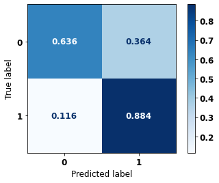
precision recall f1-score support
0 0.550 0.636 0.590 3944
1 0.916 0.884 0.900 17745
accuracy 0.839 21689
macro avg 0.733 0.760 0.745 21689
weighted avg 0.850 0.839 0.844 21689
Random Forest SP for years 2008 to 2011
[ ]:
display_confusion_matrix(rf_sp_08_11, X_testSP_12_15, y_testSP_12_15)
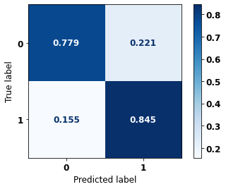
precision recall f1-score support
0 0.495 0.779 0.605 5442
1 0.951 0.845 0.895 27842
accuracy 0.834 33284
macro avg 0.723 0.812 0.750 33284
weighted avg 0.877 0.834 0.848 33284
[ ]:
display_confusion_matrix(rf_sp_08_11, X_testSP_16_21, y_testSP_16_21)

precision recall f1-score support
0 0.489 0.769 0.598 3944
1 0.941 0.821 0.877 17745
accuracy 0.812 21689
macro avg 0.715 0.795 0.737 21689
weighted avg 0.859 0.812 0.826 21689
XGBoost SP for years 2008 to 2011
[ ]:
display_confusion_matrix(xgb_sp_08_11, X_testSP_12_15, y_testSP_12_15)

precision recall f1-score support
0 0.523 0.744 0.614 5442
1 0.945 0.867 0.905 27842
accuracy 0.847 33284
macro avg 0.734 0.806 0.759 33284
weighted avg 0.876 0.847 0.857 33284
[ ]:
display_confusion_matrix(xgb_sp_08_11, X_testSP_16_21, y_testSP_16_21)

precision recall f1-score support
0 0.534 0.699 0.606 3944
1 0.928 0.865 0.895 17745
accuracy 0.835 21689
macro avg 0.731 0.782 0.751 21689
weighted avg 0.857 0.835 0.843 21689
Random Forest SP for years 2012 to 2015
[ ]:
display_confusion_matrix(rf_sp_12_15, X_testSP_16_21, y_testSP_16_21)

precision recall f1-score support
0 0.478 0.815 0.603 3944
1 0.951 0.802 0.870 17745
accuracy 0.805 21689
macro avg 0.715 0.809 0.737 21689
weighted avg 0.865 0.805 0.822 21689
XGBoost SP for years 2012 to 2015
[ ]:
display_confusion_matrix(xgb_sp_12_15, X_testSP_16_21, y_testSP_16_21)
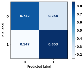
precision recall f1-score support
0 0.528 0.742 0.617 3944
1 0.937 0.853 0.893 17745
accuracy 0.832 21689
macro avg 0.733 0.797 0.755 21689
weighted avg 0.863 0.832 0.843 21689
Random Forest Other states for years 2000 to 2003
[ ]:
display_confusion_matrix(rf_fora_00_03, X_testOS_04_07, y_testOS_04_07)
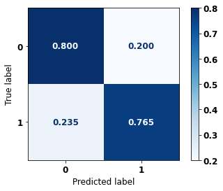
precision recall f1-score support
0 0.429 0.800 0.558 225
1 0.946 0.765 0.846 1021
accuracy 0.771 1246
macro avg 0.687 0.782 0.702 1246
weighted avg 0.852 0.771 0.794 1246
[ ]:
display_confusion_matrix(rf_fora_00_03, X_testOS_08_11, y_testOS_08_11)

precision recall f1-score support
0 0.456 0.837 0.590 264
1 0.960 0.795 0.870 1287
accuracy 0.802 1551
macro avg 0.708 0.816 0.730 1551
weighted avg 0.874 0.802 0.822 1551
[ ]:
display_confusion_matrix(rf_fora_00_03, X_testOS_12_15, y_testOS_12_15)

precision recall f1-score support
0 0.422 0.877 0.570 292
1 0.974 0.796 0.876 1715
accuracy 0.808 2007
macro avg 0.698 0.836 0.723 2007
weighted avg 0.894 0.808 0.832 2007
[ ]:
display_confusion_matrix(rf_fora_00_03, X_testOS_16_20, y_testOS_16_20)

precision recall f1-score support
0 0.433 0.832 0.570 304
1 0.956 0.770 0.853 1438
accuracy 0.781 1742
macro avg 0.695 0.801 0.711 1742
weighted avg 0.865 0.781 0.803 1742
XGBoost Other states for years 2000 to 2003
[ ]:
display_confusion_matrix(xgb_fora_00_03, X_testOS_04_07, y_testOS_04_07)

precision recall f1-score support
0 0.449 0.800 0.575 225
1 0.947 0.784 0.857 1021
accuracy 0.787 1246
macro avg 0.698 0.792 0.716 1246
weighted avg 0.857 0.787 0.806 1246
[ ]:
display_confusion_matrix(xgb_fora_00_03, X_testOS_08_11, y_testOS_08_11)

precision recall f1-score support
0 0.522 0.864 0.650 264
1 0.968 0.838 0.898 1287
accuracy 0.842 1551
macro avg 0.745 0.851 0.774 1551
weighted avg 0.892 0.842 0.856 1551
[ ]:
display_confusion_matrix(xgb_fora_00_03, X_testOS_12_15, y_testOS_12_15)

precision recall f1-score support
0 0.434 0.877 0.580 292
1 0.975 0.805 0.882 1715
accuracy 0.816 2007
macro avg 0.704 0.841 0.731 2007
weighted avg 0.896 0.816 0.838 2007
[ ]:
display_confusion_matrix(xgb_fora_00_03, X_testOS_16_20, y_testOS_16_20)

precision recall f1-score support
0 0.451 0.832 0.585 304
1 0.957 0.786 0.863 1438
accuracy 0.794 1742
macro avg 0.704 0.809 0.724 1742
weighted avg 0.869 0.794 0.814 1742
Random Forest Other states for years 2004 to 2007
[ ]:
display_confusion_matrix(rf_fora_04_07, X_testOS_08_11, y_testOS_08_11)
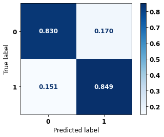
precision recall f1-score support
0 0.530 0.830 0.647 264
1 0.960 0.849 0.901 1287
accuracy 0.846 1551
macro avg 0.745 0.839 0.774 1551
weighted avg 0.887 0.846 0.858 1551
[ ]:
display_confusion_matrix(rf_fora_04_07, X_testOS_12_15, y_testOS_12_15)

precision recall f1-score support
0 0.473 0.849 0.608 292
1 0.970 0.839 0.900 1715
accuracy 0.841 2007
macro avg 0.722 0.844 0.754 2007
weighted avg 0.898 0.841 0.857 2007
[ ]:
display_confusion_matrix(rf_fora_04_07, X_testOS_16_20, y_testOS_16_20)

precision recall f1-score support
0 0.478 0.819 0.604 304
1 0.955 0.811 0.877 1438
accuracy 0.812 1742
macro avg 0.716 0.815 0.740 1742
weighted avg 0.872 0.812 0.829 1742
XGBoost Other states for years 2004 to 2007
[ ]:
display_confusion_matrix(xgb_fora_04_07, X_testOS_08_11, y_testOS_08_11)

precision recall f1-score support
0 0.537 0.848 0.658 264
1 0.965 0.850 0.904 1287
accuracy 0.850 1551
macro avg 0.751 0.849 0.781 1551
weighted avg 0.892 0.850 0.862 1551
[ ]:
display_confusion_matrix(xgb_fora_04_07, X_testOS_12_15, y_testOS_12_15)

precision recall f1-score support
0 0.483 0.853 0.617 292
1 0.971 0.845 0.904 1715
accuracy 0.846 2007
macro avg 0.727 0.849 0.760 2007
weighted avg 0.900 0.846 0.862 2007
[ ]:
display_confusion_matrix(xgb_fora_04_07, X_testOS_16_20, y_testOS_16_20)

precision recall f1-score support
0 0.477 0.829 0.606 304
1 0.957 0.808 0.876 1438
accuracy 0.812 1742
macro avg 0.717 0.819 0.741 1742
weighted avg 0.873 0.812 0.829 1742
Random Forest Other states for years 2008 to 2011
[ ]:
display_confusion_matrix(rf_fora_08_11, X_testOS_12_15, y_testOS_12_15)

precision recall f1-score support
0 0.480 0.887 0.623 292
1 0.978 0.836 0.901 1715
accuracy 0.844 2007
macro avg 0.729 0.862 0.762 2007
weighted avg 0.905 0.844 0.861 2007
[ ]:
display_confusion_matrix(rf_fora_08_11, X_testOS_16_20, y_testOS_16_20)

precision recall f1-score support
0 0.494 0.862 0.628 304
1 0.965 0.814 0.883 1438
accuracy 0.822 1742
macro avg 0.730 0.838 0.756 1742
weighted avg 0.883 0.822 0.839 1742
XGBoost Other states for years 2008 to 2011
[ ]:
display_confusion_matrix(xgb_fora_08_11, X_testOS_12_15, y_testOS_12_15)

precision recall f1-score support
0 0.481 0.853 0.615 292
1 0.971 0.843 0.903 1715
accuracy 0.845 2007
macro avg 0.726 0.848 0.759 2007
weighted avg 0.900 0.845 0.861 2007
[ ]:
display_confusion_matrix(xgb_fora_08_11, X_testOS_16_20, y_testOS_16_20)
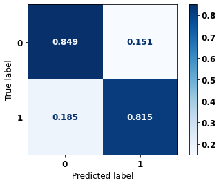
precision recall f1-score support
0 0.492 0.849 0.623 304
1 0.962 0.815 0.883 1438
accuracy 0.821 1742
macro avg 0.727 0.832 0.753 1742
weighted avg 0.880 0.821 0.837 1742
Random Forest Other states for years 2012 to 2015
[ ]:
display_confusion_matrix(rf_fora_12_15, X_testOS_16_20, y_testOS_16_20)

precision recall f1-score support
0 0.504 0.832 0.628 304
1 0.959 0.827 0.888 1438
accuracy 0.828 1742
macro avg 0.731 0.830 0.758 1742
weighted avg 0.879 0.828 0.843 1742
XGBoost Other states for years 2012 to 2015
[ ]:
display_confusion_matrix(xgb_fora_12_15, X_testOS_16_20, y_testOS_16_20)

precision recall f1-score support
0 0.505 0.832 0.629 304
1 0.959 0.828 0.888 1438
accuracy 0.828 1742
macro avg 0.732 0.830 0.758 1742
weighted avg 0.880 0.828 0.843 1742