Introduction
In this section, two machine learning models will be used to classify the obito_geral column, Random Forest and XGBoost, for both datasets, São Paulo and other states.
The label is 0 if the person is alive and 1 if he / she died.
Four scenarios will be created using the column obito_geral as label. The first is the raw data for São Paulo and other states, as was generated in the previous section. The second scenario considers only patients with morphology with the last digit being 3, in addition, the EC column was removed.
The third and fourth scenarios use the years of diagnosis grouped, the last one also considering only morphologies with the final digit 3. The years will be grouped as follows: 2000 to 2003, 2004 to 2007, 2008 to 2011, 2012 to 2015 and 2016 until the end. So we will have 5 datasets for SP and another 5 for other states.
Reading the data from SP and other states.
[ ]:
df_SP = read_csv('/content/drive/MyDrive/Trabalho/Cancer/Datasets/gearl_sp_labels.csv')
df_fora = read_csv('/content/drive/MyDrive/Trabalho/Cancer/Datasets/geral_fora_sp_labels.csv')
(506037, 77)
(32891, 77)
[ ]:
df_SP.head(3)
| SEXO | IDADE | ESCOLARI | UFRESID | IBGE | CATEATEND | CLINICA | DIAGPREV | BASEDIAG | TOPO | ... | REC03 | HABILIT2 | ULTICONS | ULTIDIAG | ULTITRAT | obito_geral | obito_cancer | vivo_ano1 | vivo_ano3 | vivo_ano5 | |
|---|---|---|---|---|---|---|---|---|---|---|---|---|---|---|---|---|---|---|---|---|---|
| 0 | 1 | 26 | 2 | SP | 3529401 | 9 | 4 | 1 | 3 | C491 | ... | **Sem informação** | 2 | 5852 | 5738 | 5738 | 0 | 0 | 1 | 1 | 1 |
| 1 | 1 | 50 | 9 | SP | 3531209 | 2 | 26 | 2 | 3 | C402 | ... | **Sem informação** | 2 | 1293 | 1331 | 1248 | 0 | 0 | 1 | 1 | 0 |
| 2 | 1 | 23 | 9 | SP | 3542602 | 9 | 26 | 1 | 3 | C402 | ... | **Sem informação** | 1 | 2053 | 1942 | 1942 | 1 | 1 | 1 | 1 | 1 |
3 rows × 77 columns
[ ]:
df_fora.head(3)
| SEXO | IDADE | ESCOLARI | UFRESID | IBGE | CATEATEND | CLINICA | DIAGPREV | BASEDIAG | TOPO | ... | REC03 | HABILIT2 | ULTICONS | ULTIDIAG | ULTITRAT | obito_geral | obito_cancer | vivo_ano1 | vivo_ano3 | vivo_ano5 | |
|---|---|---|---|---|---|---|---|---|---|---|---|---|---|---|---|---|---|---|---|---|---|
| 0 | 1 | 26 | 4 | AC | 1200401 | 2 | 24 | 2 | 3 | C402 | ... | **Sem informação** | 2 | 669 | 710 | 594 | 0 | 0 | 1 | 0 | 0 |
| 1 | 1 | 49 | 3 | BA | 2930709 | 2 | 26 | 1 | 3 | C402 | ... | **Sem informação** | 2 | 3163 | 3055 | 2893 | 0 | 0 | 1 | 1 | 1 |
| 2 | 1 | 59 | 9 | MG | 3102605 | 9 | 32 | 1 | 3 | C619 | ... | **Sem informação** | 2 | 1967 | 1967 | 1770 | 0 | 0 | 1 | 1 | 1 |
3 rows × 77 columns
[ ]:
# SP
df_SP.isna().sum().sort_values(ascending=False).head(6)
SEXO         0
IMUNOAPOS    0
FAIXAETAR    0
ANODIAG      0
DIAGTRAT     0
TRATCONS     0
dtype: int64
[ ]:
# Other states
df_fora.isna().sum().sort_values(ascending=False).head(6)
SEXO         0
IMUNOAPOS    0
FAIXAETAR    0
ANODIAG      0
DIAGTRAT     0
TRATCONS     0
dtype: int64
Here we have the correlations between the label and the other columns, the columns with higher correlations will not be used as features of the models, because they may have been used to create the label, such as the ULTINFO column, or they can be used as label for other machine learning models.
[ ]:
# SP
corr_matrix = df_SP.corr()
abs(corr_matrix['obito_geral']).sort_values(ascending = False).head(20)
obito_geral     1.000000
ULTINFO         0.866060
obito_cancer    0.778975
vivo_ano3       0.365068
ULTIDIAG        0.340122
ULTICONS        0.336685
ULTITRAT        0.332492
vivo_ano5       0.294475
vivo_ano1       0.288888
ANODIAG         0.264297
CIRURGIA        0.260995
QUIMIO          0.226548
CATEATEND       0.220804
RECNENHUM       0.208701
MORFO           0.195059
IDADE           0.190838
RECREGIO        0.153588
GLEASON         0.152939
PSA             0.152179
SEXO            0.150677
Name: obito_geral, dtype: float64
[ ]:
# Other states
corr_matrix = df_fora.corr()
abs(corr_matrix['obito_geral']).sort_values(ascending = False).head(20)
obito_geral     1.000000
ULTINFO         0.866780
obito_cancer    0.847824
vivo_ano3       0.385518
ULTIDIAG        0.350399
ULTICONS        0.343164
ULTITRAT        0.338123
CIRURGIA        0.301963
vivo_ano5       0.301465
vivo_ano1       0.281608
QUIMIO          0.252260
ANODIAG         0.228325
CATEATEND       0.222303
MORFO           0.182062
GLEASON         0.151939
PSA             0.149539
ESCOLARI        0.142043
HORMONIO        0.141135
DIAGTRAT        0.135024
RECNENHUM       0.129595
Name: obito_geral, dtype: float64
Here we have the number of examples for each category of the label, it is possible to notice that there is an imbalance.
[ ]:
df_SP.obito_geral.value_counts()
0    276947
1    229090
Name: obito_geral, dtype: int64
[ ]:
df_fora.obito_geral.value_counts()
0    20359
1    12532
Name: obito_geral, dtype: int64
First approach
Approach with “raw data”.
Preprocessing
Now we are going to divide the data into training and testing, and then do the preprocessing in both datasets to perform the training of the models and their evaluation.
First, it is necessary to define the columns that will be used as features and the label. We will not use some columns of the data: UFRESID, because we already have the division between SP and other states in the two datasets.
It was chosen to keep the column IDADE, so we will not use the FAIXAETAR. Finally, the other columns contained in the list list_drop are possible labels, so they will not be used as features for machine learning models.
[ ]:
list_drop = ['UFRESID', 'FAIXAETAR', 'ULTICONS', 'ULTIDIAG', 'ULTITRAT',
             'vivo_ano1', 'vivo_ano3', 'vivo_ano5', 'ULTINFO', 'obito_cancer']

lb = 'obito_geral'
A function was created to perform the preprocessing, preprocessing, that uses the other functions created, get_train_test (divides the dataset into train and test sets), train_preprocessing (do the preprocessing of the train set) and test_preprocessing (do the preprocessing of the test set).
To see the complete function go to the functions section.
SP
[ ]:
X_train_SP, X_test_SP, y_train_SP, y_test_SP, feat_cols_SP = preprocessing(df_SP, list_drop, lb,
                                                                           random_state=seed,
                                                                           balance_data=False,
                                                                           encoder_type='LabelEncoder',
                                                                           norm_name='StandardScaler')
X_train = (379527, 66), X_test = (126510, 66)
y_train = (379527,), y_test = (126510,)
Other states
[ ]:
X_train_OS, X_test_OS, y_train_OS, y_test_OS, feat_cols_OS = preprocessing(df_fora, list_drop, lb,
                                                                           random_state=seed,
                                                                           balance_data=False,
                                                                           encoder_type='LabelEncoder',
                                                                           norm_name='StandardScaler')
X_train = (24668, 66), X_test = (8223, 66)
y_train = (24668,), y_test = (8223,)
Training machine learning models
After dividing the data into training and testing, using the encoder and normalizing, the data is ready to be used by the machine learning models.
Random Forest
The first model that will be tested is the Random Forest, for this test the parameter random_state will be used, to obtain the same training values of the model every time it is runned.
The hyperparameter class_weight was also used, because teh model has difficulty learning the class with fewer examples, so using this parameter this class will have a higher weight in the training of the model.
[ ]:
# SP
rf_sp = RandomForestClassifier(class_weight={0:1, 1:1.272},
                               random_state=seed,
                               criterion='entropy',
                               max_depth=10)

rf_sp.fit(X_train_SP, y_train_SP)
RandomForestClassifier(class_weight={0: 1, 1: 1.272}, criterion='entropy',
                       max_depth=10, random_state=10)
[ ]:
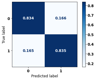
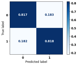
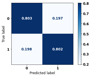
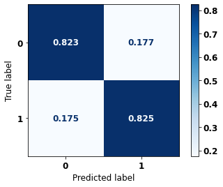
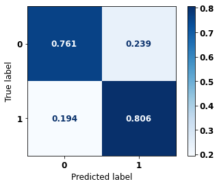
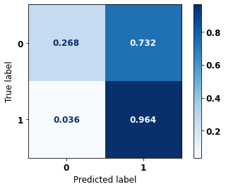
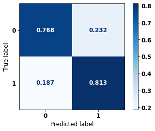
display_confusion_matrix(rf_sp, X_test_SP, y_test_SP)
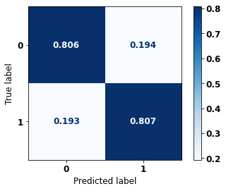
              precision    recall  f1-score   support

           0      0.834     0.806     0.820     69237
           1      0.774     0.807     0.790     57273

    accuracy                          0.806    126510
   macro avg      0.804     0.806     0.805    126510
weighted avg      0.807     0.806     0.806    126510
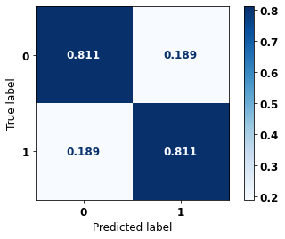
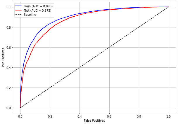
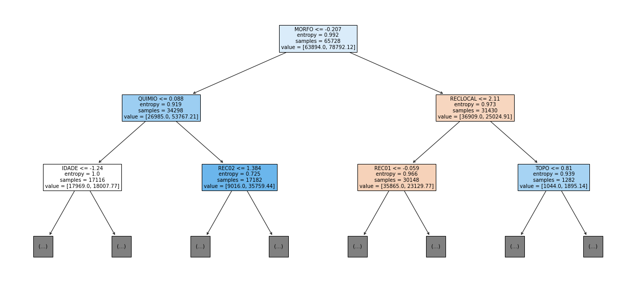
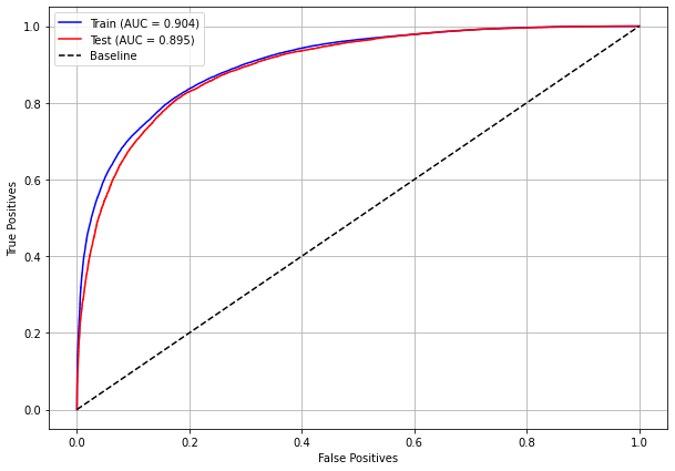
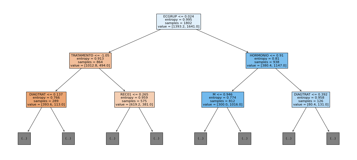
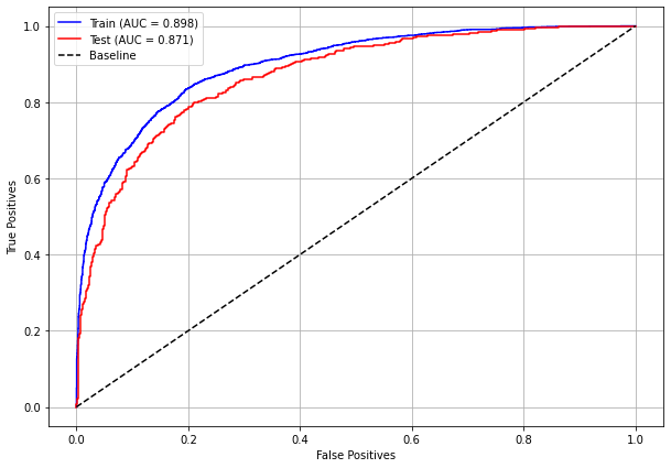
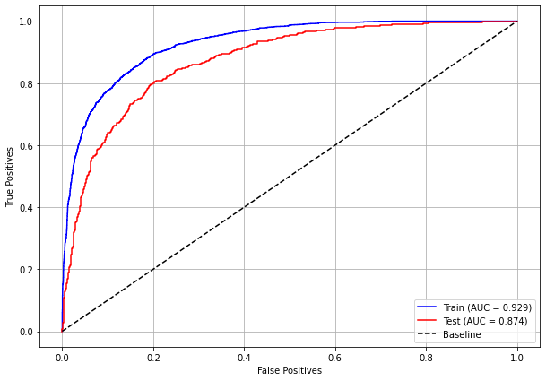
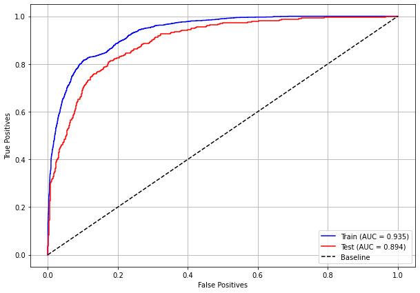
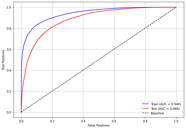
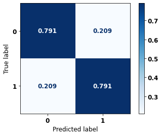
The confusion matrix obtained for the Random Forest, with SP data, shows a good performance of the model, with 81% of accuracy.
[ ]:
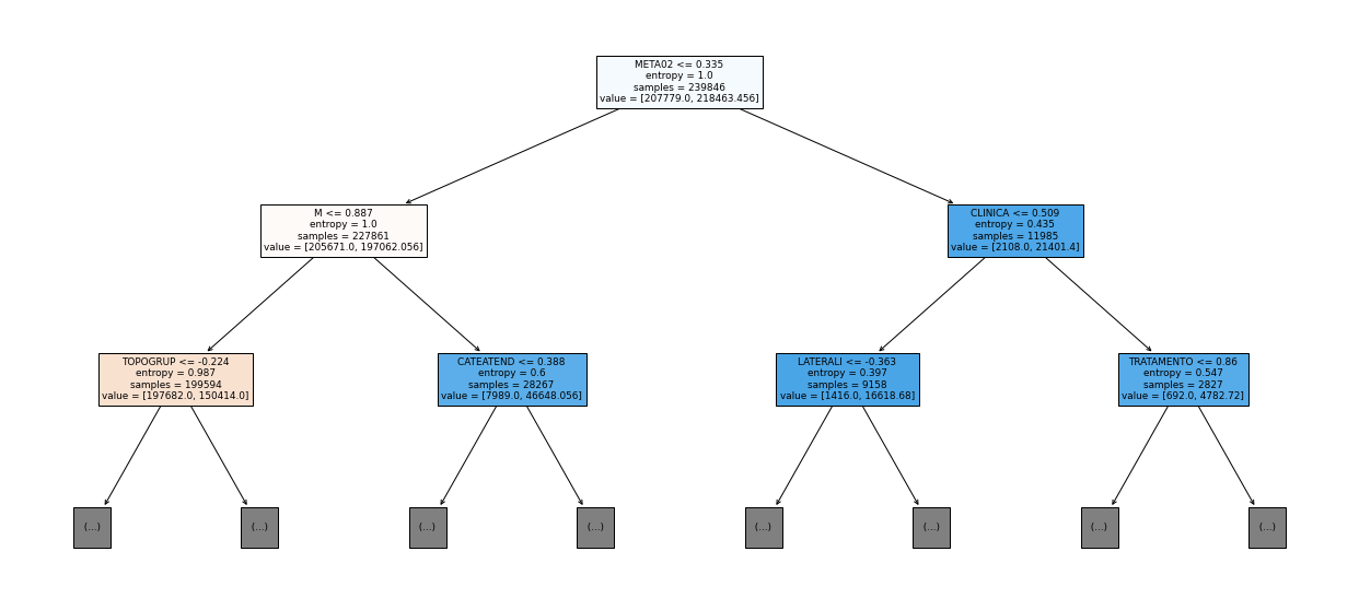
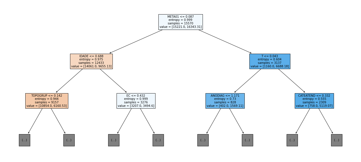
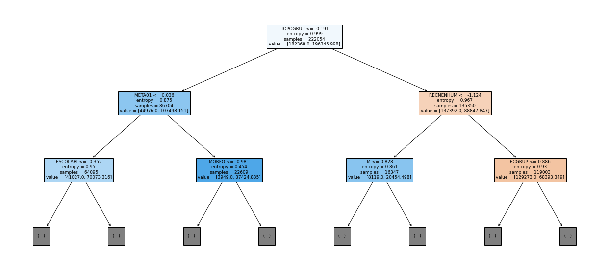
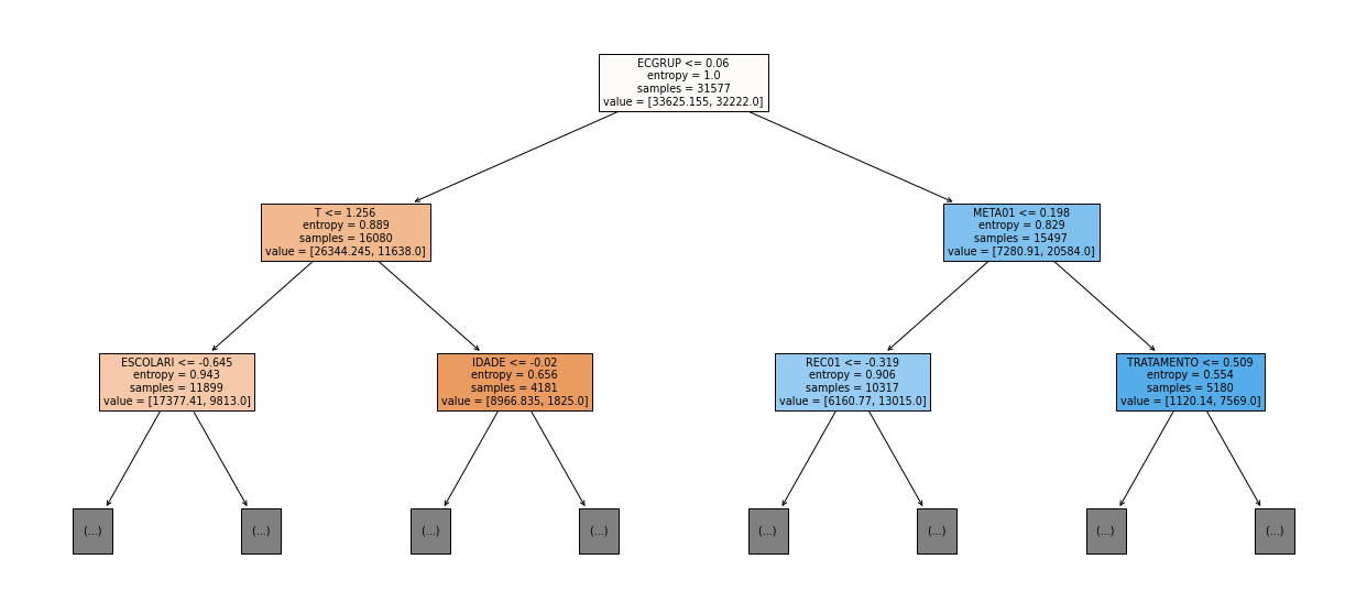
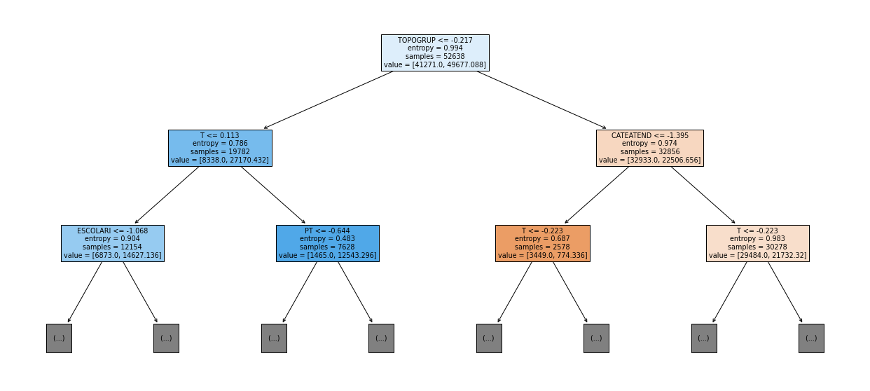
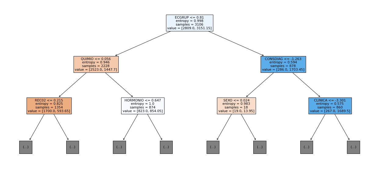
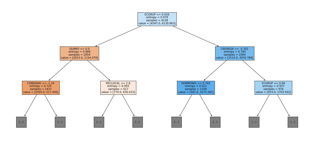
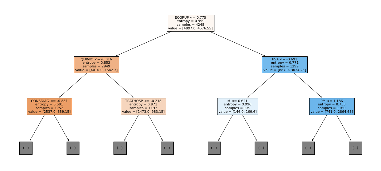
show_tree(rf_sp, feat_cols_SP, 2)
[ ]:
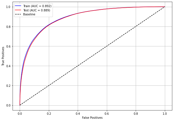
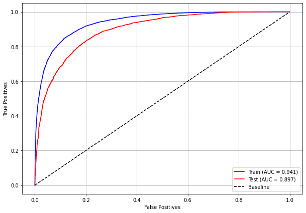
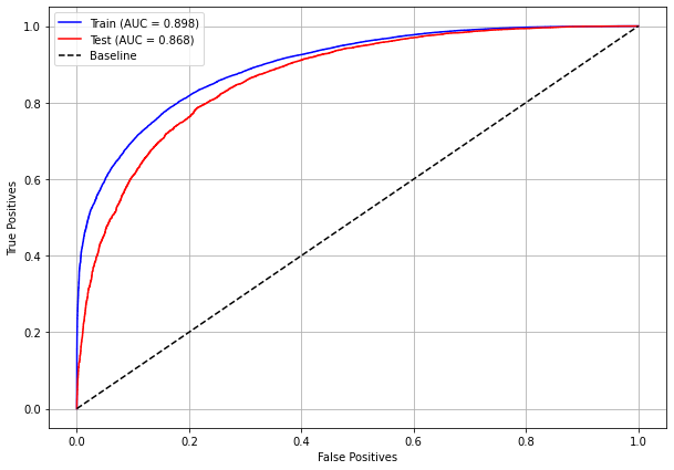
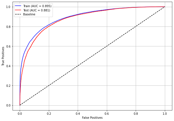
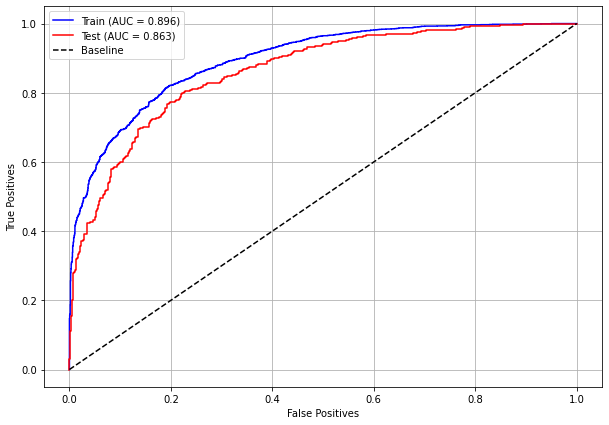
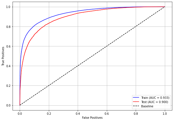
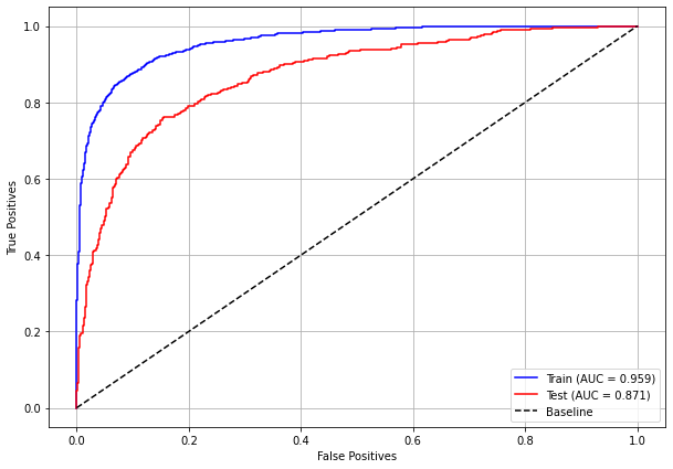
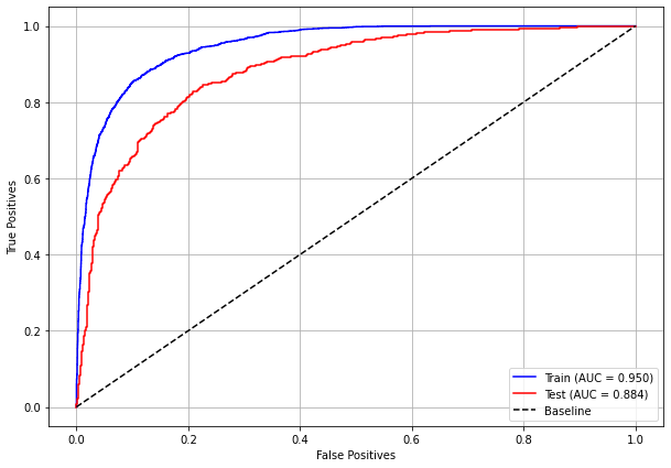
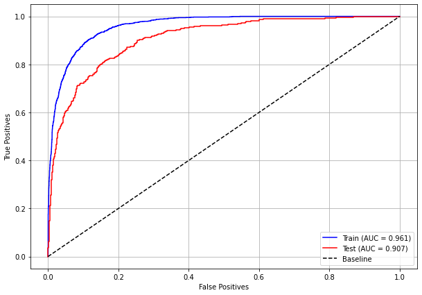
plot_roc_curve(rf_sp, X_train_SP, X_test_SP, y_train_SP, y_test_SP)
[ ]:
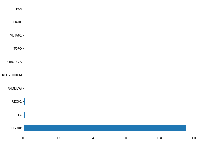
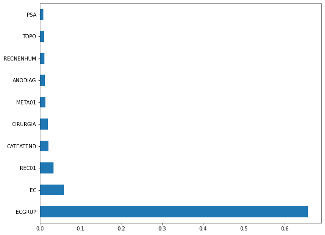
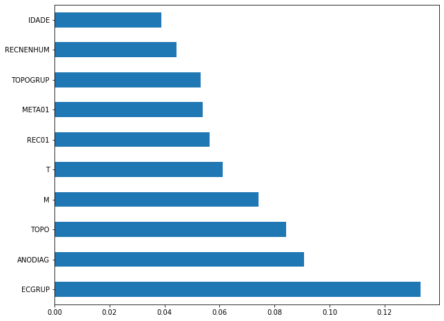
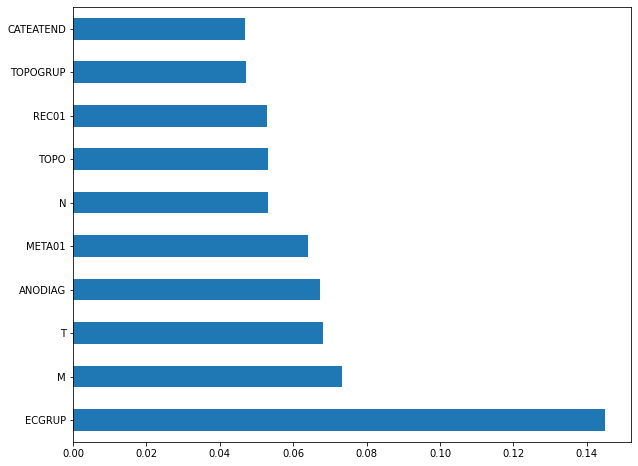
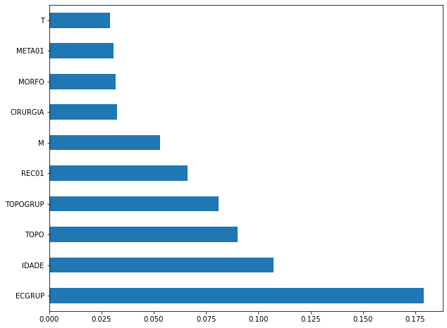
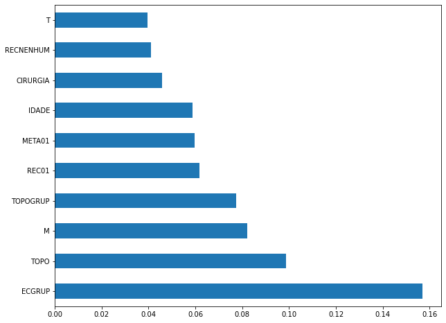
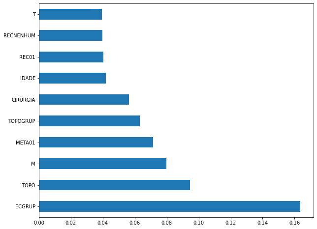
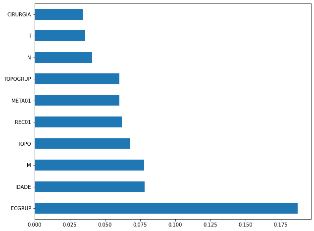
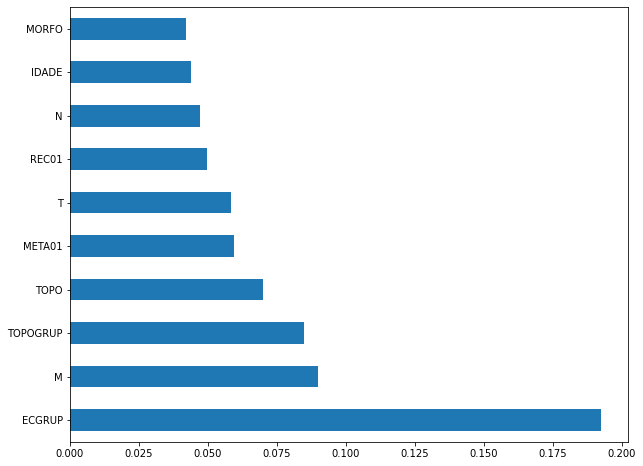
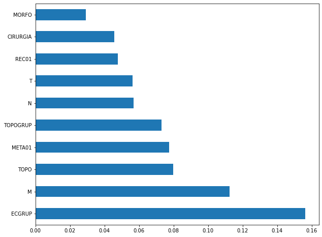
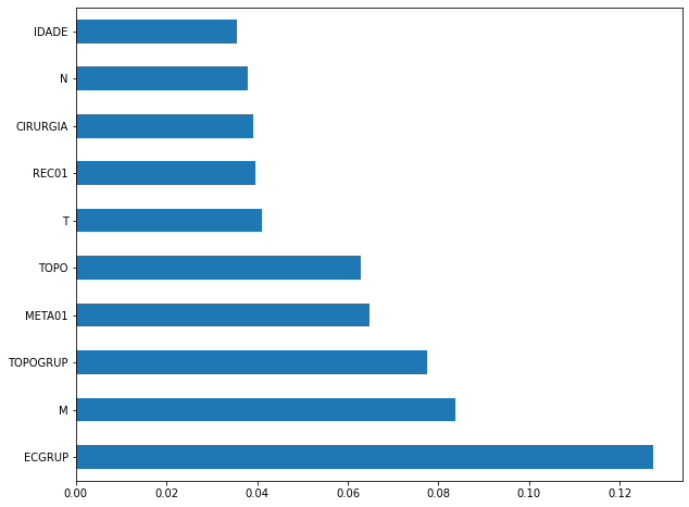
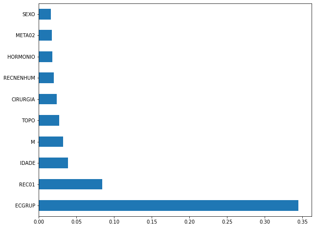
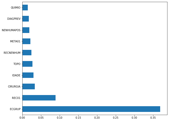
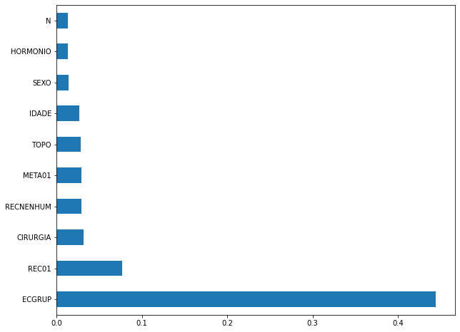
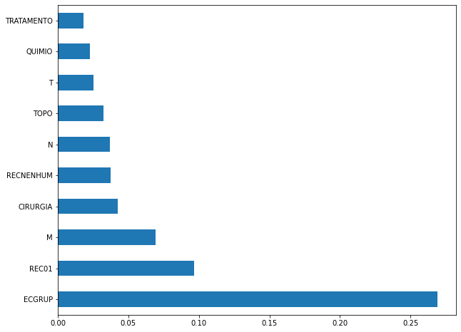
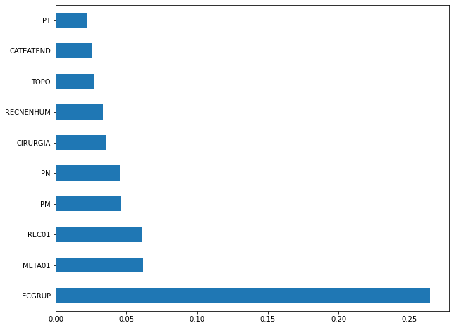
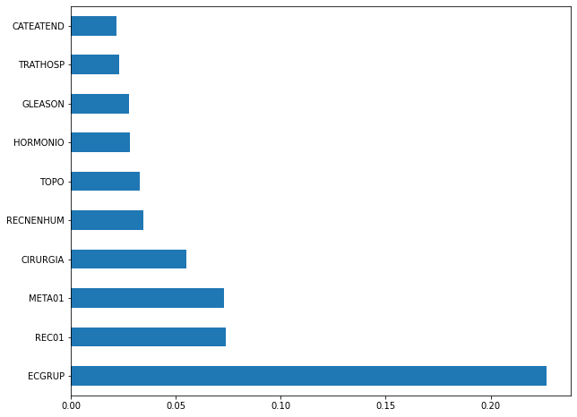
plot_feat_importances(rf_sp, feat_cols_SP)
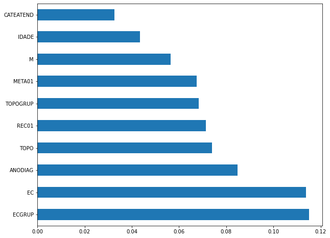
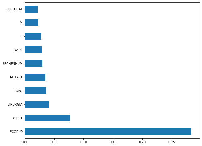
The four most important features in the model were
ECGRUP,EC,ANODIAGandTOPO.
[ ]:
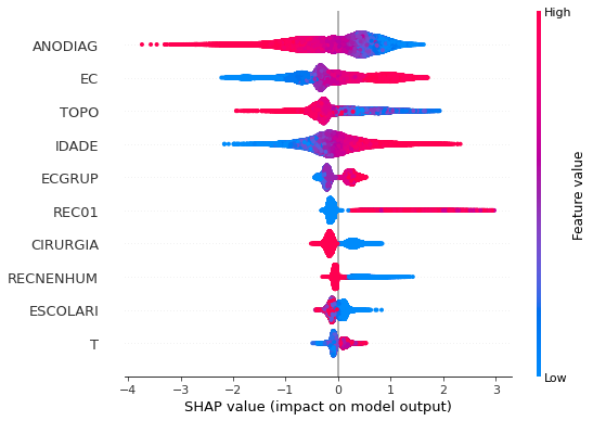
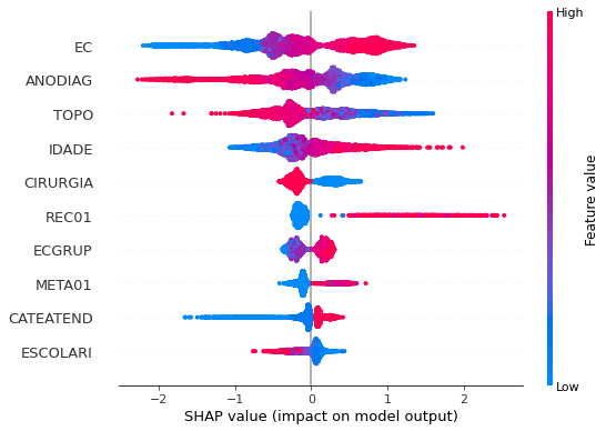
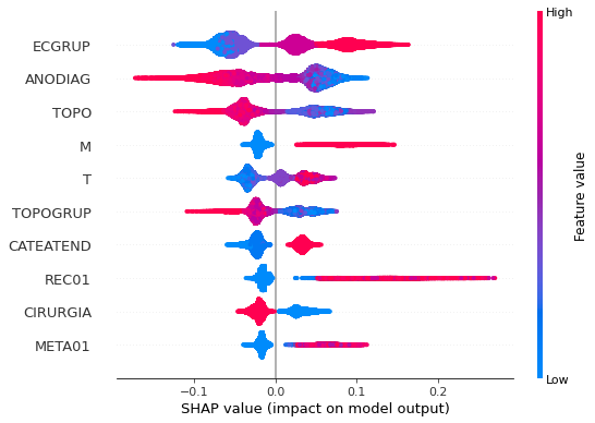
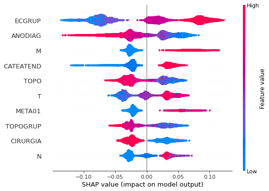
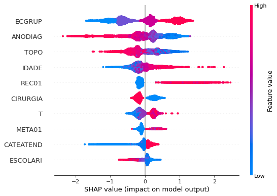
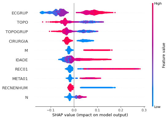
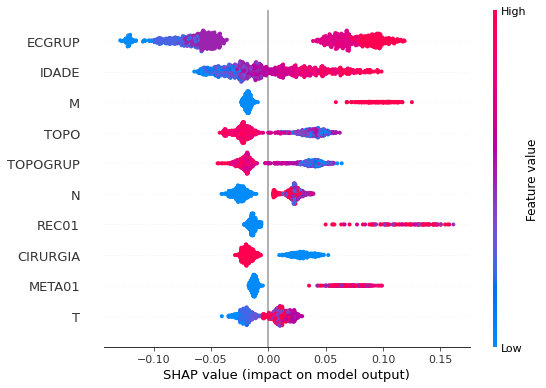
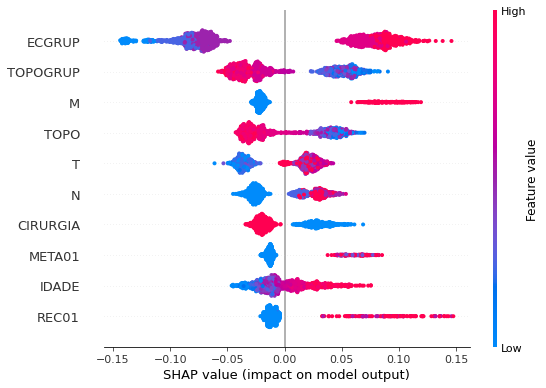
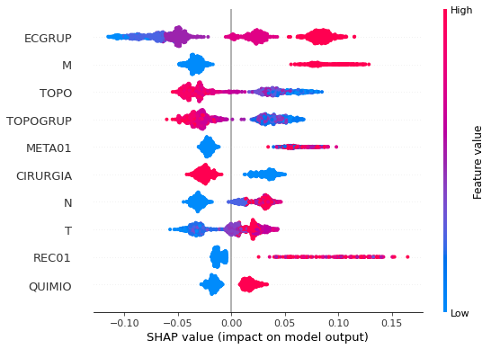
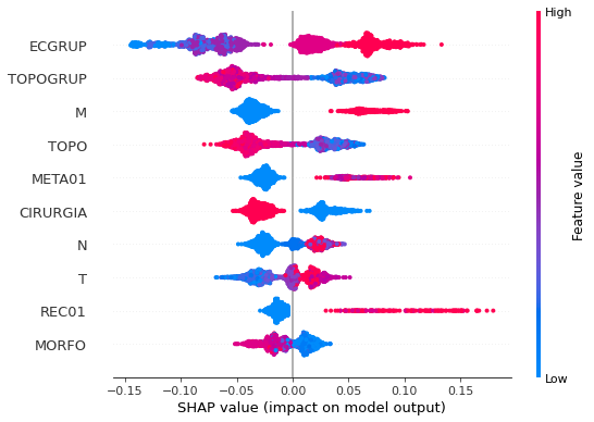
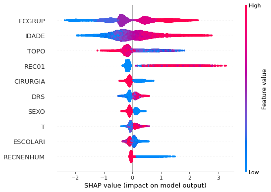
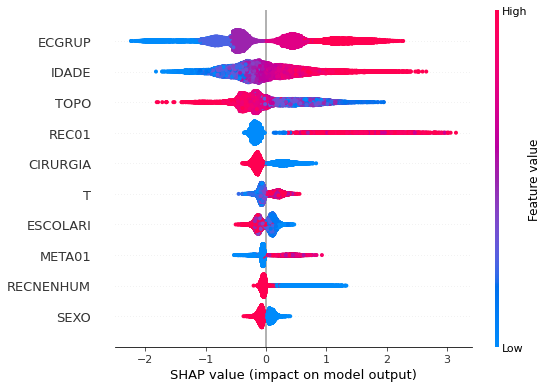
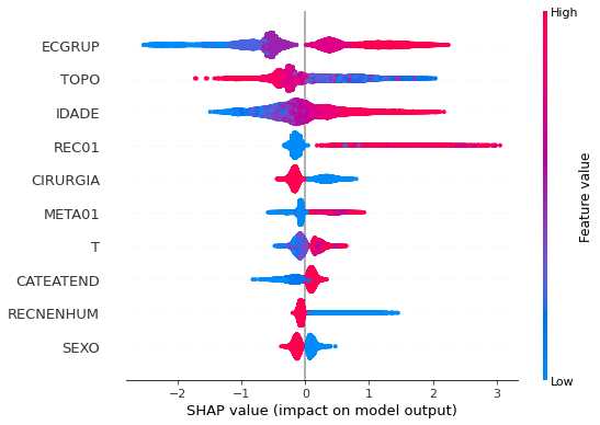
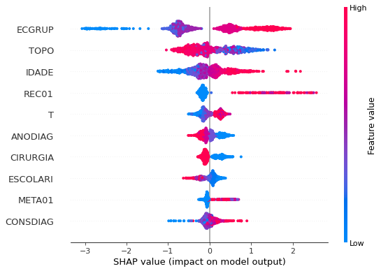
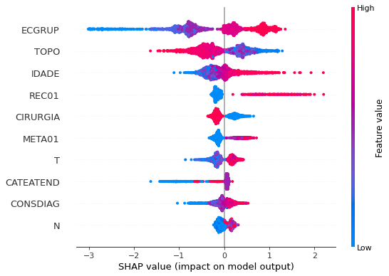
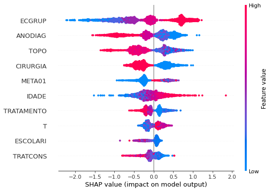
plot_shap_values(rf_sp, X_test_SP, feat_cols_SP)
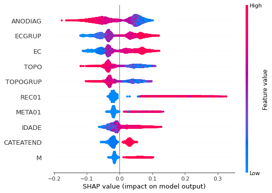
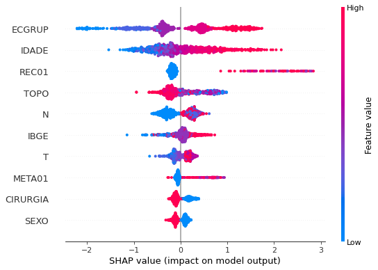
Note that larger values of the ANODIAG column, shown in pink, have more influence for the model’s prediction to be class 0, smaller values have greater weight for the prediction to be class 1.
The other columns shown follow the same logic.
[ ]:
# Other states
rf_fora = RandomForestClassifier(class_weight={0:1, 1:1.73},
                                 random_state=seed,
                                 criterion='entropy',
                                 max_depth=8)

rf_fora.fit(X_train_OS, y_train_OS)
RandomForestClassifier(class_weight={0: 1, 1: 1.73}, criterion='entropy',
                       max_depth=8, random_state=10)
[ ]:
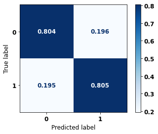
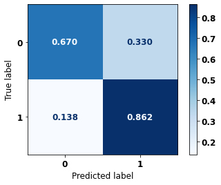
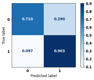
display_confusion_matrix(rf_fora, X_test_OS, y_test_OS)

              precision    recall  f1-score   support

           0      0.863     0.794     0.827      5090
           1      0.704     0.795     0.747      3133

    accuracy                          0.795      8223
   macro avg      0.783     0.795     0.787      8223
weighted avg      0.802     0.795     0.797      8223
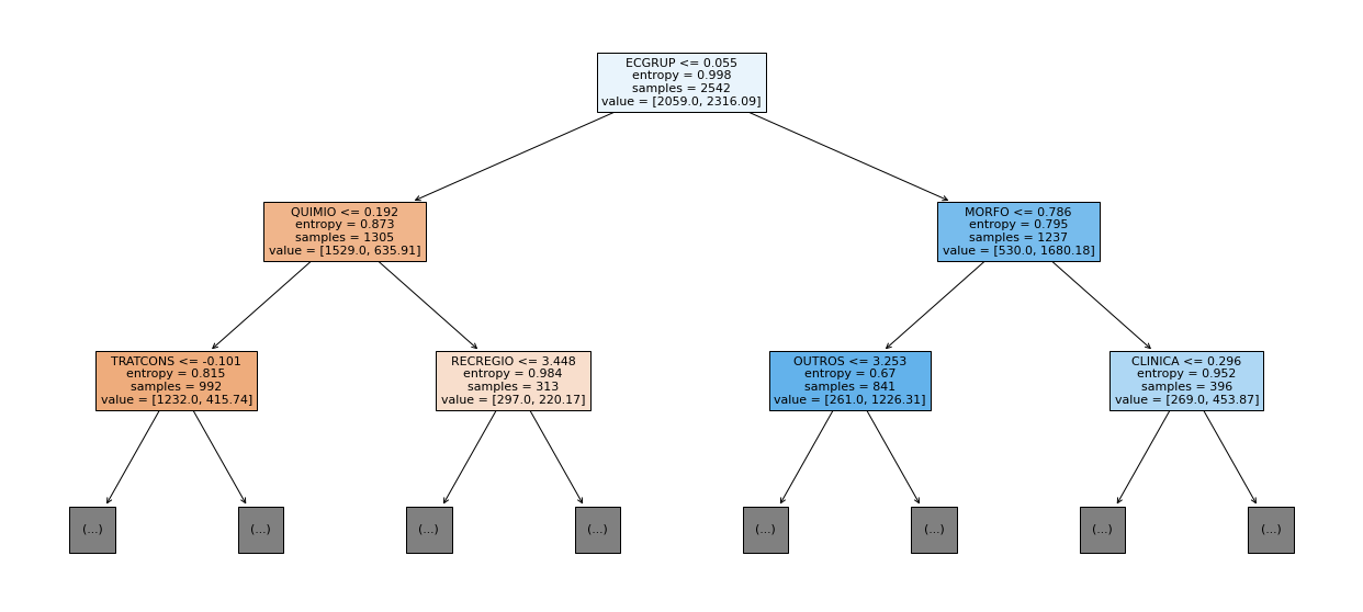
The confusion matrix obtained for the Random Forest algorithm, with other states data, shows a good performance of the model, because the model achieves a 79% of accuracy.
[ ]:
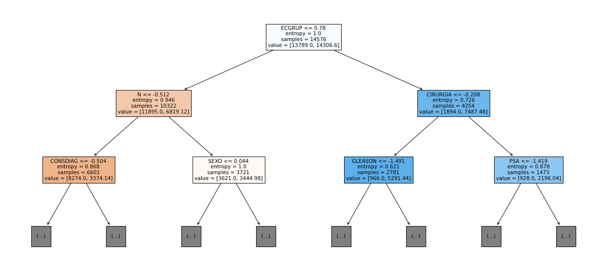
show_tree(rf_fora, feat_cols_OS, 2)
[ ]:
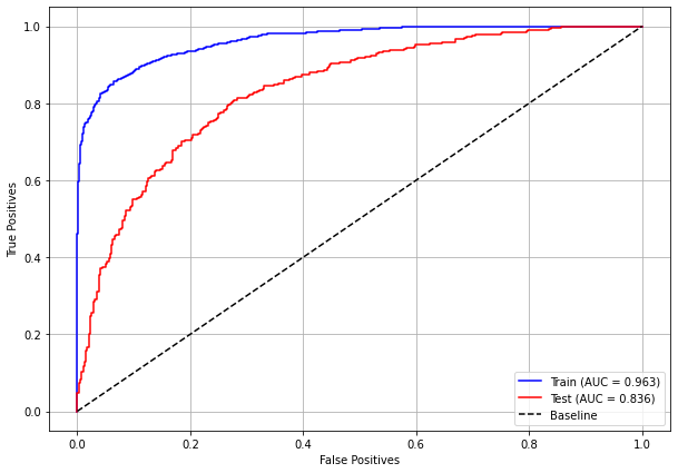
plot_roc_curve(rf_fora, X_train_OS, X_test_OS, y_train_OS, y_test_OS)

[ ]:
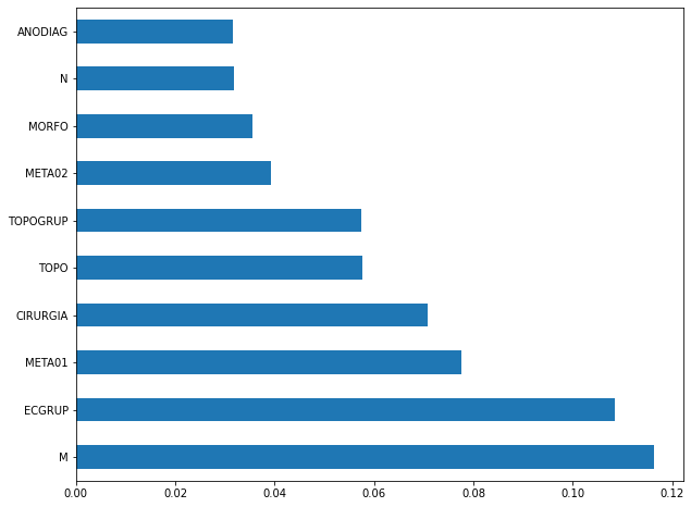
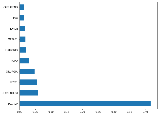
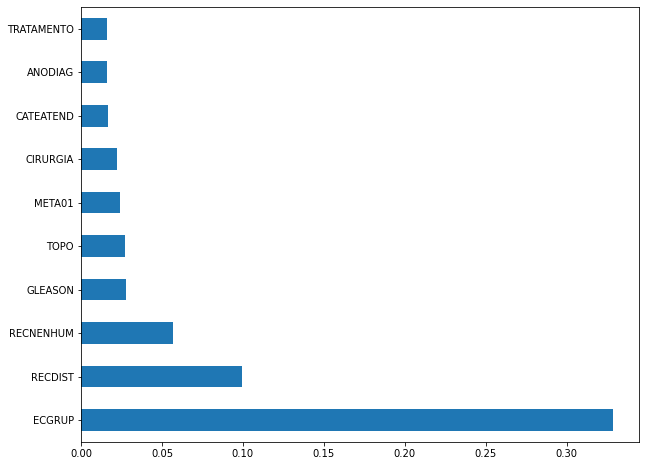
plot_feat_importances(rf_fora, feat_cols_OS)
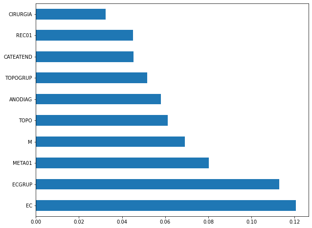
The four most important features in the model were
EC,ECGRUP,META01andM.
[ ]:
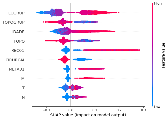
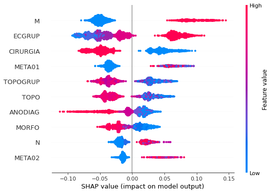
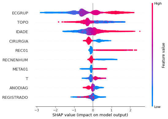
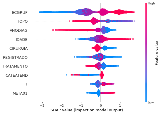
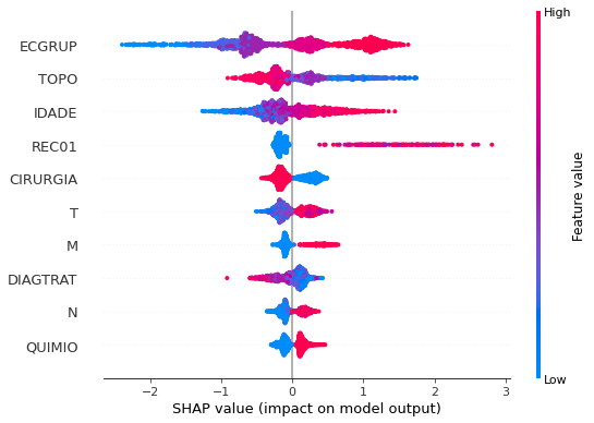
plot_shap_values(rf_fora, X_test_OS, feat_cols_OS)
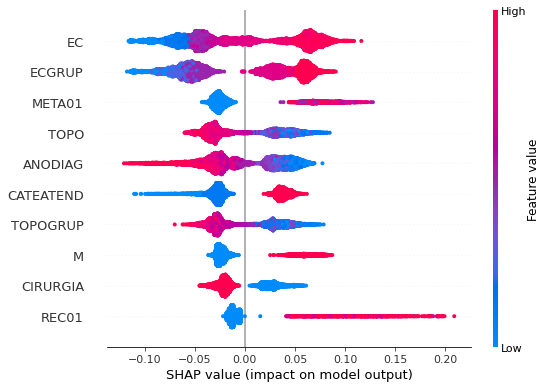
Note that larger values of the EC column, shown in pink, have more influence for the model’s prediction to be class 1, smaller values have greater weight for the prediction to be class 0. This behavior was expected, because the higher the clinical stage, worse is the stage of cancer.
The other columns shown follow the same logic.
Randomized Grid Search
[ ]:
# RandomizedSearchCV
hyperRF = {'n_estimators': [100, 150, 200, 250],
           'max_depth': [5, 8, 10, 12, 15],
           'min_samples_split': [2, 5, 10, 15],
           'min_samples_leaf': [1, 2, 5, 10]}

rf = RandomForestClassifier(random_state=seed, criterion='entropy')

randRS = RandomizedSearchCV(rf, hyperRF, n_iter=20, cv=5, n_jobs=-1,
                            random_state=seed)
[ ]:
# SP
bestSP = randRS.fit(X_train_SP, y_train_SP)
[ ]:
bestSP.best_params_
{'n_estimators': 200,
 'min_samples_split': 10,
 'min_samples_leaf': 2,
 'max_depth': 15}
[ ]:
# SP
rf_sp_opt = bestSP.best_estimator_
rf_sp_opt.set_params(class_weight={0:1, 1:1.25})

rf_sp_opt.fit(X_train_SP, y_train_SP)
RandomForestClassifier(class_weight={0: 1, 1: 1.25}, criterion='entropy',
                       max_depth=15, min_samples_leaf=2, min_samples_split=10,
                       n_estimators=200, random_state=10)
[ ]:
display_confusion_matrix(rf_sp_opt, X_test_SP, y_test_SP)

              precision    recall  f1-score   support

           0      0.847     0.820     0.833     69237
           1      0.790     0.820     0.805     57273

    accuracy                          0.820    126510
   macro avg      0.819     0.820     0.819    126510
weighted avg      0.821     0.820     0.820    126510
[ ]:
# Other States
bestOS = randRS.fit(X_train_OS, y_train_OS)
[ ]:
bestOS.best_params_
{'n_estimators': 200,
 'min_samples_split': 10,
 'min_samples_leaf': 2,
 'max_depth': 15}
[ ]:
# Other states
rf_fora_opt = bestOS.best_estimator_
rf_fora_opt.set_params(class_weight={0:1, 1:2.1})

rf_fora_opt.fit(X_train_OS, y_train_OS)
RandomForestClassifier(class_weight={0: 1, 1: 2.1}, criterion='entropy',
                       max_depth=15, min_samples_leaf=2, min_samples_split=10,
                       n_estimators=200, random_state=10)
[ ]:
display_confusion_matrix(rf_fora_opt, X_test_OS, y_test_OS)
              precision    recall  f1-score   support

           0      0.874     0.811     0.842      5090
           1      0.725     0.811     0.766      3133

    accuracy                          0.811      8223
   macro avg      0.800     0.811     0.804      8223
weighted avg      0.818     0.811     0.813      8223
XGBoost
The training of the XGBoost model follows the same pattern with random_state. A higher weight was also used for the class with fewer examples, using the hyperparameter scale_pos_weight.
The hyperparameter max_depth was chosen as 10 because the default value for this hyperparameter is 3, a low value for the amount of data we have.
[ ]:
# SP
xgboost_sp = XGBClassifier(max_depth=10,
                           scale_pos_weight=1.25,
                           random_state=seed)

xgboost_sp.fit(X_train_SP, y_train_SP)
XGBClassifier(max_depth=10, random_state=10, scale_pos_weight=1.25)
[ ]:
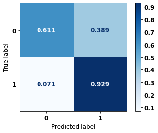
display_confusion_matrix(xgboost_sp, X_test_SP, y_test_SP)

              precision    recall  f1-score   support

           0      0.857     0.832     0.844     69237
           1      0.804     0.832     0.818     57273

    accuracy                          0.832    126510
   macro avg      0.830     0.832     0.831    126510
weighted avg      0.833     0.832     0.832    126510
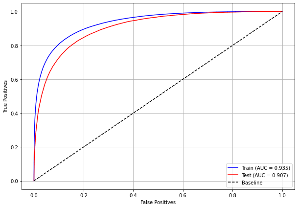
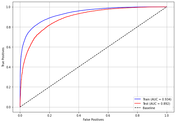
The confusion matrix obtained for the XGBoost, with SP data, shows a good performance of the model, with 83% of accuracy.
[ ]:
plot_roc_curve(xgboost_sp, X_train_SP, X_test_SP, y_train_SP, y_test_SP)

[ ]:
plot_feat_importances(xgboost_sp, feat_cols_SP)
The four most important features in the model were
ECGRUP,EC,REC01andANODIAG.
[ ]:
plot_shap_values(xgboost_sp, X_test_SP, feat_cols_SP)
Note that larger values of the ANODIAG column, shown in pink, have more influence for the model’s prediction to be class 0, smaller values have greater weight for the prediction to be class 1.
The other columns shown follow the same logic.
[ ]:
# Other states
xgboost_fora = XGBClassifier(max_depth=6,
                             scale_pos_weight=1.68,
                             random_state=seed)

xgboost_fora.fit(X_train_OS, y_train_OS)
XGBClassifier(max_depth=6, random_state=10, scale_pos_weight=1.68)
[ ]:
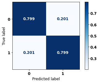
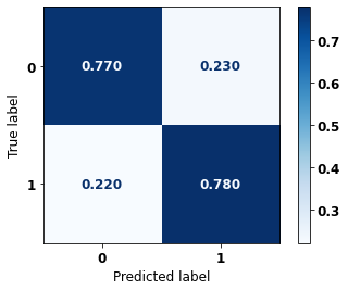
display_confusion_matrix(xgboost_fora, X_test_OS, y_test_OS)

              precision    recall  f1-score   support

           0      0.878     0.815     0.845      5090
           1      0.731     0.816     0.771      3133

    accuracy                          0.815      8223
   macro avg      0.804     0.816     0.808      8223
weighted avg      0.822     0.815     0.817      8223
The confusion matrix obtained for the XGBoost algorithm, with other states data, shows a good performance of the model, because the model achieves a 81% of accuracy.
[ ]:
plot_roc_curve(xgboost_fora, X_train_OS, X_test_OS, y_train_OS, y_test_OS)
[ ]:
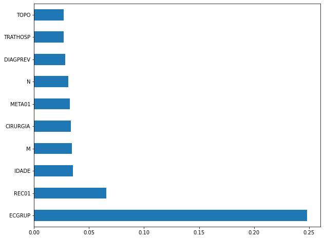
plot_feat_importances(xgboost_fora, feat_cols_OS)
The four most important features in the model were
ECGRUP,EC,REC01andCATEATEND.
[ ]:
plot_shap_values(xgboost_fora, X_test_OS, feat_cols_OS)
Note that larger values of the EC column, shown in pink, have more influence for the model’s prediction to be class 1, smaller values have greater weight for the prediction to be class 0. This behavior was expected, because the higher the clinical stage, worse is the stage of cancer.
The other columns shown follow the same logic.
Randomized Grid Search
[ ]:
# RandomizedSearchCV
hyperXGB = {'learning_rate': [0.05, 0.10, 0.15, 0.20],
            'max_depth': [5, 8, 10, 12, 15],
            'min_child_weight': [1, 3, 5, 7],
            'gamma': [0.0, 0.1, 0.2 , 0.3],
            'colsample_bytree': [0.3, 0.4, 0.5, 0.7],
            'n_estimators': [100, 150, 200, 250]}

xgboost = XGBClassifier(random_state=seed)
xgbRS = RandomizedSearchCV(xgboost, hyperXGB, n_iter=20, cv=5, n_jobs=-1,
                           random_state=seed)
[ ]:
# SP
bestSP = xgbRS.fit(X_train_SP, y_train_SP)
[ ]:
bestSP.best_params_
{'n_estimators': 200,
 'min_child_weight': 5,
 'max_depth': 10,
 'learning_rate': 0.1,
 'gamma': 0.2,
 'colsample_bytree': 0.4}
[ ]:
# SP
xgb_sp_opt = bestSP.best_estimator_
xgb_sp_opt.set_params(scale_pos_weight=1.26)

xgb_sp_opt.fit(X_train_SP, y_train_SP)
XGBClassifier(colsample_bytree=0.4, gamma=0.2, max_depth=10, min_child_weight=5,
              n_estimators=200, random_state=10, scale_pos_weight=1.26)
[ ]:
display_confusion_matrix(xgb_sp_opt, X_test_SP, y_test_SP)
              precision    recall  f1-score   support

           0      0.860     0.834     0.847     69237
           1      0.806     0.835     0.820     57273

    accuracy                          0.835    126510
   macro avg      0.833     0.835     0.833    126510
weighted avg      0.835     0.835     0.835    126510
[ ]:
# Other States
bestOS = xgbRS.fit(X_train_OS, y_train_OS)
[ ]:
bestOS.best_params_
{'n_estimators': 150,
 'min_child_weight': 7,
 'max_depth': 8,
 'learning_rate': 0.05,
 'gamma': 0.2,
 'colsample_bytree': 0.4}
[ ]:
# Other states
xgb_fora_opt = bestOS.best_estimator_
xgb_fora_opt.set_params(scale_pos_weight=1.76)

xgb_fora_opt.fit(X_train_OS, y_train_OS)
XGBClassifier(colsample_bytree=0.4, gamma=0.2, learning_rate=0.05, max_depth=8,
              min_child_weight=7, n_estimators=150, random_state=10,
              scale_pos_weight=1.76)
[ ]:
display_confusion_matrix(xgb_fora_opt, X_test_OS, y_test_OS)

              precision    recall  f1-score   support

           0      0.879     0.818     0.848      5090
           1      0.735     0.817     0.774      3133

    accuracy                          0.818      8223
   macro avg      0.807     0.818     0.811      8223
weighted avg      0.824     0.818     0.820      8223
Second approach
Approach using only morphologies with final digit equal to 3 and without EC column as a feature.
Preprocessing
Now we are going to divide the data into training and testing, and then do the preprocessing in both datasets to perform the training of the models and their evaluation.
First, it is necessary to define the columns that will be used as features and the label. We will not use some columns of the data: UFRESID, because we already have the division between SP and other states in the two datasets.
It was chosen to keep the column IDADE, so we will not use the FAIXAETAR, as well as the column ECGRUP and not the column EC. Finally, the other columns contained in the list list_drop are possible labels, so they will not be used as features for machine learning models.
[ ]:
list_drop = ['UFRESID', 'FAIXAETAR', 'ULTICONS', 'ULTIDIAG', 'ULTITRAT',
             'vivo_ano1', 'vivo_ano3', 'vivo_ano5', 'ULTINFO', 'EC', 'obito_cancer']

lb = 'obito_geral'
A function was created to perform the preprocessing, preprocessing, that uses the other functions created, get_train_test (divides the dataset into train and test sets), train_preprocessing (do the preprocessing of the train set) and test_preprocessing (do the preprocessing of the test set).
To see the complete function go to the functions section.
SP
[ ]:
X_train_SP, X_test_SP, y_train_SP, y_test_SP, feat_cols_SP = preprocessing(df_SP, list_drop, lb,
                                                                           morpho3=True,
                                                                           random_state=seed,
                                                                           balance_data=False,
                                                                           encoder_type='LabelEncoder',
                                                                           norm_name='StandardScaler')
X_train = (351486, 65), X_test = (117163, 65)
y_train = (351486,), y_test = (117163,)
Other states
[ ]:
X_train_OS, X_test_OS, y_train_OS, y_test_OS, feat_cols_OS = preprocessing(df_fora, list_drop, lb,
                                                                           morpho3=True,
                                                                           random_state=seed,
                                                                           balance_data=False,
                                                                           encoder_type='LabelEncoder',
                                                                           norm_name='StandardScaler')
X_train = (23079, 65), X_test = (7693, 65)
y_train = (23079,), y_test = (7693,)
Training machine learning models
After dividing the data into training and testing, using the encoder and normalizing, the data is ready to be used by the machine learning models.
Random Forest
The first model that will be tested is the Random Forest, for this test the parameter random_state will be used, to obtain the same training values of the model every time it is runned.
The hyperparameter class_weight was also used, because the model has difficulty learning the class with fewer examples, so using this parameter this class will have a higher weight in the training of the model.
[ ]:
# SP
rf_sp = RandomForestClassifier(random_state=seed,
                               class_weight={0:1, 1:1.161},
                               criterion='entropy',
                               max_depth=10)

rf_sp.fit(X_train_SP, y_train_SP)
RandomForestClassifier(class_weight={0: 1, 1: 1.161}, criterion='entropy',
                       max_depth=10, random_state=10)
[ ]:
display_confusion_matrix(rf_sp, X_test_SP, y_test_SP)
              precision    recall  f1-score   support

           0      0.811     0.799     0.805     60836
           1      0.786     0.799     0.793     56327

    accuracy                          0.799    117163
   macro avg      0.799     0.799     0.799    117163
weighted avg      0.799     0.799     0.799    117163
The confusion matrix obtained for the Random Forest, with SP data, also shows a good performance of the model, with 80% of accuracy.
[ ]:
show_tree(rf_sp, feat_cols_SP, 2)
[ ]:
plot_roc_curve(rf_sp, X_train_SP, X_test_SP, y_train_SP, y_test_SP)

[ ]:
plot_feat_importances(rf_sp, feat_cols_SP)
The four most important features in the model were
ECGRUP,ANODIAG,TOPOandM.
[ ]:
plot_shap_values(rf_sp, X_test_SP, feat_cols_SP)
Note that larger values of the ECGRUP column, shown in pink, have more influence for the model’s prediction to be class 1, smaller values have greater weight for the prediction to be class 0. This behavior was expected, because the higher the clinical stage, worse is the stage of cancer.
The other columns shown follow the same logic.
[ ]:
# Other states
rf_fora = RandomForestClassifier(random_state=seed,
                                 class_weight={0:1, 1:1.54},
                                 criterion='entropy',
                                 max_depth=8)

rf_fora.fit(X_train_OS, y_train_OS)
RandomForestClassifier(class_weight={0: 1, 1: 1.54}, criterion='entropy',
                       max_depth=8, random_state=10)
[ ]:
display_confusion_matrix(rf_fora, X_test_OS, y_test_OS)

              precision    recall  f1-score   support

           0      0.848     0.791     0.819      4588
           1      0.719     0.791     0.753      3105

    accuracy                          0.791      7693
   macro avg      0.784     0.791     0.786      7693
weighted avg      0.796     0.791     0.792      7693
The confusion matrix obtained for the Random Forest algorithm with other states data shows a good performance of the model, because the model achieves a 79% of accuracy.
[ ]:
show_tree(rf_fora, feat_cols_OS, 2)
[ ]:
plot_roc_curve(rf_fora, X_train_OS, X_test_OS, y_train_OS, y_test_OS)
[ ]:
plot_feat_importances(rf_fora, feat_cols_OS)
The four most important features in the model were
ECGRUP,M,TandANODIAG.
[ ]:
plot_shap_values(rf_fora, X_test_OS, feat_cols_OS)
Note that larger values of the ECGRUP column, shown in pink, have more influence for the model’s prediction to be class 1, smaller values have greater weight for the prediction to be class 0. This behavior was expected, because the higher the clinical stage, worse is the stage of cancer.
The other columns shown follow the same logic.
XGBoost
The training of the XGBoost model follows the same pattern with random_state. A higher weight was also used for the class with fewer examples, using the hyperparameter scale_pos_weight.
The hyperparameter max_depth was chosen as 10 because the default value for this hyperparameter is 3, a low value for the amount of data we have.
[ ]:
# SP
xgboost_sp = XGBClassifier(max_depth=10,
                           scale_pos_weight=1.13,
                           random_state=seed)

xgboost_sp.fit(X_train_SP, y_train_SP)
XGBClassifier(max_depth=10, random_state=10, scale_pos_weight=1.13)
[ ]:
display_confusion_matrix(xgboost_sp, X_test_SP, y_test_SP)

              precision    recall  f1-score   support

           0      0.836     0.826     0.831     60836
           1      0.815     0.825     0.820     56327

    accuracy                          0.826    117163
   macro avg      0.825     0.826     0.825    117163
weighted avg      0.826     0.826     0.826    117163
The confusion matrix obtained for the XGBoost, with SP data, also shows a good performance of the model, with 83% of accuracy.
[ ]:
plot_roc_curve(xgboost_sp, X_train_SP, X_test_SP, y_train_SP, y_test_SP)
[ ]:
plot_feat_importances(xgboost_sp, feat_cols_SP)
The four most important features in the model were
ECGRUP,REC01,RECNENHUMandANODIAG.
[ ]:
plot_shap_values(xgboost_sp, X_test_SP, feat_cols_SP)
Note that larger values of the ECGRUP column, shown in pink, have more influence for the model’s prediction to be class 1, smaller values have greater weight for the prediction to be class 0. This behavior was expected, because the higher the clinical stage, worse is the stage of cancer.
The other columns shown follow the same logic.
[ ]:
# Other states
xgboost_fora = XGBClassifier(max_depth=6,
                             scale_pos_weight=1.471,
                             random_state=seed)

xgboost_fora.fit(X_train_OS, y_train_OS)
XGBClassifier(max_depth=6, random_state=10, scale_pos_weight=1.471)
[ ]:
display_confusion_matrix(xgboost_fora, X_test_OS, y_test_OS)

              precision    recall  f1-score   support

           0      0.862     0.810     0.836      4588
           1      0.743     0.809     0.774      3105

    accuracy                          0.810      7693
   macro avg      0.802     0.810     0.805      7693
weighted avg      0.814     0.810     0.811      7693
The confusion matrix obtained for the XGBoost algorithm with SP data shows a good performance of the model, because the model achieves a 81% of accuracy.
[ ]:
plot_roc_curve(xgboost_fora, X_train_OS, X_test_OS, y_train_OS, y_test_OS)
[ ]:
plot_feat_importances(xgboost_fora, feat_cols_OS)
The four most important features in the model were
ECGRUP,REC01,CATEATENDandMETA01.
[ ]:
plot_shap_values(xgboost_fora, X_test_OS, feat_cols_OS)
Note that larger values of the ECGRUP column, shown in pink, have more influence for the model’s prediction to be class 1, smaller values have greater weight for the prediction to be class 0. This behavior was expected, because the higher the clinical stage, worse is the stage of cancer.
The other columns shown follow the same logic.
Third approach
Approach with grouped years and without the column EC.
Preprocessing
Now we are going to divide the data into training and testing, and then do the preprocessing in both datasets to perform the training of the models and their evaluation. We will use the years grouped too, resulting in 5 datasets for SP and more 5 for other states.
First, it is necessary to define the columns that will be used as features and the label. We will not use some columns of the data: UFRESID, because we already have the division between SP and other states in the two datasets.
It was chosen to keep the column IDADE, so we will not use the FAIXAETAR, as well as the column ECGRUP and not the column EC. Finally, the other columns contained in the list list_drop are possible labels, so they will not be used as features for machine learning models.
[ ]:
list_drop = ['UFRESID', 'FAIXAETAR', 'ULTICONS', 'ULTIDIAG', 'ULTITRAT',
             'vivo_ano1', 'vivo_ano3', 'vivo_ano5', 'ULTINFO', 'EC', 'obito_cancer']

lb = 'obito_geral'
A function was created to perform the preprocessing, preprocessing, that uses the other functions created, get_train_test (divides the dataset into train and test sets), train_preprocessing (do the preprocessing of the train set) and test_preprocessing (do the preprocessing of the test set).
The process will be done 5 times for SP and other states, using the datasets with grouped years.
To see the complete function go to the functions section.
SP
[ ]:
X_trainSP_00_03, X_testSP_00_03, y_trainSP_00_03, y_testSP_00_03, feat_SP_00_03 = preprocessing(df_SP, list_drop, lb,
                                                                                                group_years=True,
                                                                                                first_year=2000,
                                                                                                last_year=2003,
                                                                                                random_state=seed,
                                                                                                balance_data=False,
                                                                                                encoder_type='LabelEncoder',
                                                                                                norm_name='StandardScaler')
X_train = (49873, 65), X_test = (16625, 65)
y_train = (49873,), y_test = (16625,)
[ ]:
X_trainSP_04_07, X_testSP_04_07, y_trainSP_04_07, y_testSP_04_07, feat_SP_04_07 = preprocessing(df_SP, list_drop, lb,
                                                                                                group_years=True,
                                                                                                first_year=2004,
                                                                                                last_year=2007,
                                                                                                random_state=seed,
                                                                                                balance_data=False,
                                                                                                encoder_type='LabelEncoder',
                                                                                                norm_name='StandardScaler')
X_train = (62658, 65), X_test = (20887, 65)
y_train = (62658,), y_test = (20887,)
[ ]:
X_trainSP_08_11, X_testSP_08_11, y_trainSP_08_11, y_testSP_08_11, feat_SP_08_11 = preprocessing(df_SP, list_drop, lb,
                                                                                                group_years=True,
                                                                                                first_year=2008,
                                                                                                last_year=2011,
                                                                                                random_state=seed,
                                                                                                balance_data=False,
                                                                                                encoder_type='LabelEncoder',
                                                                                                norm_name='StandardScaler')
X_train = (83228, 65), X_test = (27743, 65)
y_train = (83228,), y_test = (27743,)
[ ]:
X_trainSP_12_15, X_testSP_12_15, y_trainSP_12_15, y_testSP_12_15, feat_SP_12_15 = preprocessing(df_SP, list_drop, lb,
                                                                                                group_years=True,
                                                                                                first_year=2012,
                                                                                                last_year=2015,
                                                                                                random_state=seed,
                                                                                                balance_data=False,
                                                                                                encoder_type='LabelEncoder',
                                                                                                norm_name='StandardScaler')
X_train = (103890, 65), X_test = (34630, 65)
y_train = (103890,), y_test = (34630,)
[ ]:
X_trainSP_16_21, X_testSP_16_21, y_trainSP_16_21, y_testSP_16_21, feat_SP_16_21 = preprocessing(df_SP, list_drop, lb,
                                                                                                group_years=True,
                                                                                                first_year=2016,
                                                                                                last_year=2021,
                                                                                                random_state=seed,
                                                                                                balance_data=False,
                                                                                                encoder_type='LabelEncoder',
                                                                                                norm_name='StandardScaler')
X_train = (79877, 65), X_test = (26626, 65)
y_train = (79877,), y_test = (26626,)
Other states
[ ]:
X_trainOS_00_03, X_testOS_00_03, y_trainOS_00_03, y_testOS_00_03, feat_OS_00_03 = preprocessing(df_fora, list_drop, lb,
                                                                                                group_years=True,
                                                                                                first_year=2000,
                                                                                                last_year=2003,
                                                                                                random_state=seed,
                                                                                                balance_data=False,
                                                                                                encoder_type='LabelEncoder',
                                                                                                norm_name='StandardScaler')
X_train = (2802, 65), X_test = (935, 65)
y_train = (2802,), y_test = (935,)
[ ]:
X_trainOS_04_07, X_testOS_04_07, y_trainOS_04_07, y_testOS_04_07, feat_OS_04_07 = preprocessing(df_fora, list_drop, lb,
                                                                                                group_years=True,
                                                                                                first_year=2004,
                                                                                                last_year=2007,
                                                                                                random_state=seed,
                                                                                                balance_data=False,
                                                                                                encoder_type='LabelEncoder',
                                                                                                norm_name='StandardScaler')
X_train = (3942, 65), X_test = (1315, 65)
y_train = (3942,), y_test = (1315,)
[ ]:
X_trainOS_08_11, X_testOS_08_11, y_trainOS_08_11, y_testOS_08_11, feat_OS_08_11 = preprocessing(df_fora, list_drop, lb,
                                                                                                group_years=True,
                                                                                                first_year=2008,
                                                                                                last_year=2011,
                                                                                                random_state=seed,
                                                                                                balance_data=False,
                                                                                                encoder_type='LabelEncoder',
                                                                                                norm_name='StandardScaler')
X_train = (4842, 65), X_test = (1614, 65)
y_train = (4842,), y_test = (1614,)
[ ]:
X_trainOS_12_15, X_testOS_12_15, y_trainOS_12_15, y_testOS_12_15, feat_OS_12_15 = preprocessing(df_fora, list_drop, lb,
                                                                                                group_years=True,
                                                                                                first_year=2012,
                                                                                                last_year=2015,
                                                                                                random_state=seed,
                                                                                                balance_data=False,
                                                                                                encoder_type='LabelEncoder',
                                                                                                norm_name='StandardScaler')
X_train = (6456, 65), X_test = (2153, 65)
y_train = (6456,), y_test = (2153,)
[ ]:
X_trainOS_16_20, X_testOS_16_20, y_trainOS_16_20, y_testOS_16_20, feat_OS_16_20 = preprocessing(df_fora, list_drop, lb,
                                                                                                group_years=True,
                                                                                                first_year=2016,
                                                                                                last_year=2020,
                                                                                                random_state=seed,
                                                                                                balance_data=False,
                                                                                                encoder_type='LabelEncoder',
                                                                                                norm_name='StandardScaler')
X_train = (6624, 65), X_test = (2208, 65)
y_train = (6624,), y_test = (2208,)
Training and evaluation of the models
After dividing the data into training and testing, using the encoder and normalizing, the data is ready to be used by the machine learning models.
Random Forest
The first model is the Random Forest, the random_state will be used as a parameter, to obtain the same training values of the model every time it is runned.
The hyperparameter class_weight was used because the models have difficulty to learn the class with fewer examples.
SP
[ ]:
# SP - 2000 to 2003
rf_sp_00_03 = RandomForestClassifier(random_state=seed,
                                     class_weight={0:1.905, 1:1},
                                     criterion='entropy',
                                     max_depth=10)

rf_sp_00_03.fit(X_trainSP_00_03, y_trainSP_00_03)
RandomForestClassifier(class_weight={0: 1.905, 1: 1}, criterion='entropy',
                       max_depth=10, random_state=10)
[ ]:
display_confusion_matrix(rf_sp_00_03, X_testSP_00_03, y_testSP_00_03)

              precision    recall  f1-score   support

           0      0.665     0.786     0.720      5851
           1      0.871     0.785     0.826     10774

    accuracy                          0.785     16625
   macro avg      0.768     0.785     0.773     16625
weighted avg      0.798     0.785     0.789     16625
The confusion matrix obtained for the Random Forest, with SP data from 2000 to 2003, shows a good performance of the model, with 78% of accuracy.
[ ]:
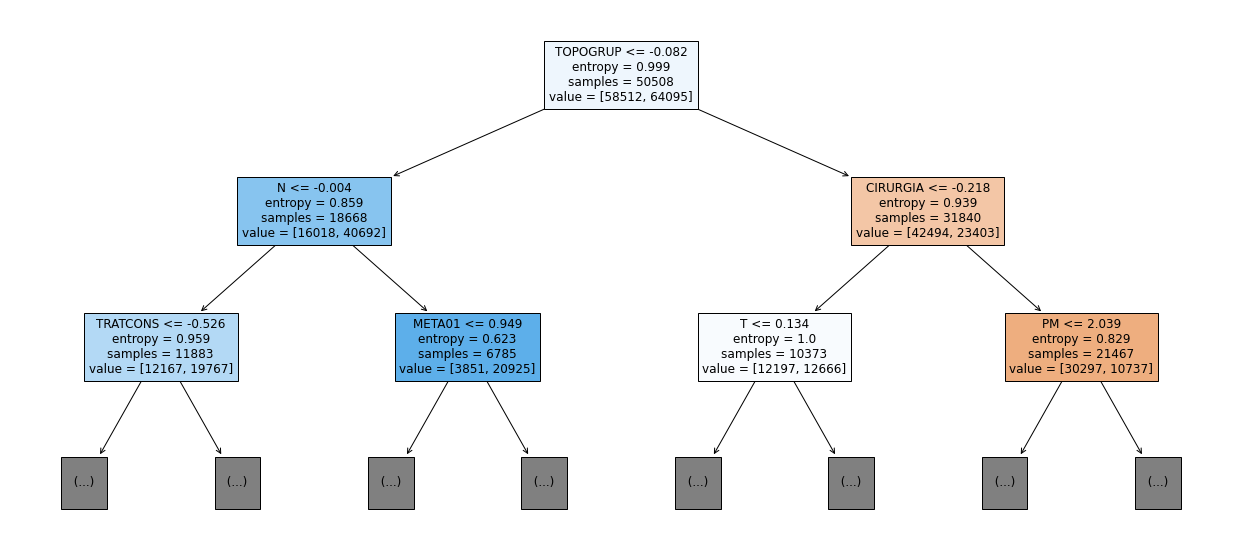
show_tree(rf_sp_00_03, feat_SP_00_03, 2)
[ ]:
plot_roc_curve(rf_sp_00_03, X_trainSP_00_03, X_testSP_00_03, y_trainSP_00_03, y_testSP_00_03)
[ ]:
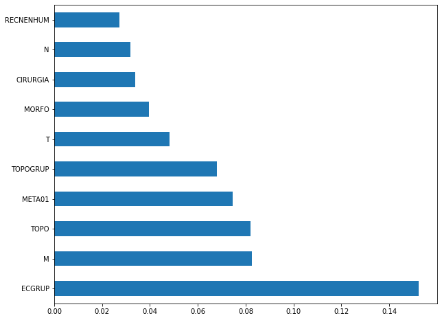
plot_feat_importances(rf_sp_00_03, feat_SP_00_03)
The four most important features in the model were
ECGRUP,IDADE,TOPO, andTOPOGRUP.
[ ]:
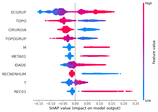
plot_shap_values(rf_sp_00_03, X_testSP_00_03, feat_SP_00_03)
Note that larger values of the ECGRUP column, shown in pink, have more influence for the model’s prediction to be class 1, smaller values have greater weight for the prediction to be class 0. This behavior was expected, because the higher the clinical stage, worse is the stage of cancer.
The other columns shown follow the same logic.
[ ]:
# SP - 2004 to 2007
rf_sp_04_07 = RandomForestClassifier(random_state=seed,
                                     class_weight={0:1.25007, 1:1},
                                     criterion='entropy',
                                     max_depth=10)

rf_sp_04_07.fit(X_trainSP_04_07, y_trainSP_04_07)
RandomForestClassifier(class_weight={0: 1.25007, 1: 1}, criterion='entropy',
                       max_depth=10, random_state=10)
[ ]:
display_confusion_matrix(rf_sp_04_07, X_testSP_04_07, y_testSP_04_07)

              precision    recall  f1-score   support

           0      0.734     0.790     0.761      8851
           1      0.837     0.789     0.812     12036

    accuracy                          0.790     20887
   macro avg      0.785     0.790     0.787     20887
weighted avg      0.793     0.790     0.791     20887
The confusion matrix obtained for the Random Forest, with SP data from 2004 to 2007, shows a good performance of the model, with 79% of accuracy.
[ ]:
show_tree(rf_sp_04_07, feat_SP_04_07, 2)
[ ]:
plot_roc_curve(rf_sp_04_07, X_trainSP_04_07, X_testSP_04_07, y_trainSP_04_07, y_testSP_04_07)
[ ]:
plot_feat_importances(rf_sp_04_07, feat_SP_04_07)
The four most important features in the model were
ECGRUP,TOPO,IDADE, andTOPOGRUP.
[ ]:
plot_shap_values(rf_sp_04_07, X_testSP_04_07, feat_SP_04_07)
Note that larger values of the ECGRUP column, shown in pink, have more influence for the model’s prediction to be class 1, smaller values have greater weight for the prediction to be class 0. This behavior was expected, because the higher the clinical stage, worse is the stage of cancer.
The other columns shown follow the same logic.
[ ]:
# SP - 2008 to 2011
rf_sp_08_11 = RandomForestClassifier(random_state=seed,
                                     class_weight={0:1, 1:1.184},
                                     criterion='entropy',
                                     max_depth=10)

rf_sp_08_11.fit(X_trainSP_08_11, y_trainSP_08_11)
RandomForestClassifier(class_weight={0: 1, 1: 1.184}, criterion='entropy',
                       max_depth=10, random_state=10)
[ ]:
display_confusion_matrix(rf_sp_08_11, X_testSP_08_11, y_testSP_08_11)

              precision    recall  f1-score   support

           0      0.797     0.800     0.798     13681
           1      0.805     0.802     0.803     14062

    accuracy                          0.801     27743
   macro avg      0.801     0.801     0.801     27743
weighted avg      0.801     0.801     0.801     27743
The confusion matrix obtained for the Random Forest, with SP data from 2008 to 2011, shows a good performance of the model, with 80% of accuracy.
[ ]:
show_tree(rf_sp_08_11, feat_SP_08_11, 2)
[ ]:
plot_roc_curve(rf_sp_08_11, X_trainSP_08_11, X_testSP_08_11, y_trainSP_08_11, y_testSP_08_11)
[ ]:
plot_feat_importances(rf_sp_08_11, feat_SP_08_11)
The four most important features in the model were
ECGRUP,TOPO,MandTOPOGRUP.
[ ]:
plot_shap_values(rf_sp_08_11, X_testSP_08_11, feat_SP_08_11)
Note that larger values of the ECGRUP column, shown in pink, have more influence for the model’s prediction to be class 1, smaller values have greater weight for the prediction to be class 0. This behavior was expected, because the higher the clinical stage, worse is the stage of cancer.
The other columns shown follow the same logic.
[ ]:
# SP - 2012 to 2015
rf_sp_12_15 = RandomForestClassifier(random_state=seed,
                                     class_weight={0:1, 1:1.97},
                                     criterion='entropy',
                                     max_depth=10)

rf_sp_12_15.fit(X_trainSP_12_15, y_trainSP_12_15)
RandomForestClassifier(class_weight={0: 1, 1: 1.97}, criterion='entropy',
                       max_depth=10, random_state=10)
[ ]:
display_confusion_matrix(rf_sp_12_15, X_testSP_12_15, y_testSP_12_15)

              precision    recall  f1-score   support

           0      0.877     0.815     0.845     21356
           1      0.733     0.816     0.772     13274

    accuracy                          0.815     34630
   macro avg      0.805     0.815     0.808     34630
weighted avg      0.822     0.815     0.817     34630
The confusion matrix obtained for the Random Forest, with SP data from 2012 to 2015, shows a good performance of the model with 81% of accuracy.
[ ]:
show_tree(rf_sp_12_15, feat_SP_12_15, 2)
[ ]:
plot_roc_curve(rf_sp_12_15, X_trainSP_12_15, X_testSP_12_15, y_trainSP_12_15, y_testSP_12_15)
[ ]:
plot_feat_importances(rf_sp_12_15, feat_SP_12_15)
The four most important features in the model were
ECGRUP,TOPO,MandMETA01.
[ ]:
plot_shap_values(rf_sp_12_15, X_testSP_12_15, feat_SP_12_15)
Note that larger values of the ECGRUP column, shown in pink, have more influence for the model’s prediction to be class 1, smaller values have greater weight for the prediction to be class 0. This behavior was expected, because the higher the clinical stage, worse is the stage of cancer.
The other columns shown follow the same logic.
[ ]:
# SP - 2016 to 2021
rf_sp_16_21 = RandomForestClassifier(random_state=seed,
                                     class_weight={0:1, 1:3},
                                     criterion='entropy',
                                     max_depth=10)

rf_sp_16_21.fit(X_trainSP_16_21, y_trainSP_16_21)
RandomForestClassifier(class_weight={0: 1, 1: 3}, criterion='entropy',
                       max_depth=10, random_state=10)
[ ]:
display_confusion_matrix(rf_sp_16_21, X_testSP_16_21, y_testSP_16_21)

              precision    recall  f1-score   support

           0      0.920     0.808     0.861     19497
           1      0.606     0.808     0.693      7129

    accuracy                          0.808     26626
   macro avg      0.763     0.808     0.777     26626
weighted avg      0.836     0.808     0.816     26626
The confusion matrix obtained for the Random Forest, with SP data from 2016 to 2021, shows a good performance of the model, with 81% of accuracy.
[ ]:
show_tree(rf_sp_16_21, feat_SP_16_21, 2)
[ ]:
plot_roc_curve(rf_sp_16_21, X_trainSP_16_21, X_testSP_16_21, y_trainSP_16_21, y_testSP_16_21)

[ ]:
plot_feat_importances(rf_sp_16_21, feat_SP_16_21)
The four most important features in the model were
ECGRUP,M,TOPO, andMETA01.
[ ]:
plot_shap_values(rf_sp_16_21, X_testSP_16_21, feat_SP_16_21)
Note that larger values of the ECGRUP column, shown in pink, have more influence for the model’s prediction to be class 1, smaller values have greater weight for the prediction to be class 0. This behavior was expected, because the higher the clinical stage, worse is the stage of cancer.
The other columns shown follow the same logic.
Other states
[ ]:
# Other states - 2000 to 2003
rf_fora_00_03 = RandomForestClassifier(random_state=seed,
                                       class_weight={0:1.2, 1:1},
                                       criterion='entropy',
                                       max_depth=6)

rf_fora_00_03.fit(X_trainOS_00_03, y_trainOS_00_03)
RandomForestClassifier(class_weight={0: 1.2, 1: 1}, criterion='entropy',
                       max_depth=6, random_state=10)
[ ]:
display_confusion_matrix(rf_fora_00_03, X_testOS_00_03, y_testOS_00_03)

              precision    recall  f1-score   support

           0      0.709     0.768     0.737       396
           1      0.818     0.768     0.792       539

    accuracy                          0.768       935
   macro avg      0.763     0.768     0.765       935
weighted avg      0.772     0.768     0.769       935
The confusion matrix obtained for the Random Forest, with other states data from 2000 to 2003, also shows a good performance of the model, and we have a balanced main diagonal with 77% of accuracy.
[ ]:
show_tree(rf_fora_00_03, feat_OS_00_03, 2)
[ ]:
plot_roc_curve(rf_fora_00_03, X_trainOS_00_03, X_testOS_00_03, y_trainOS_00_03, y_testOS_00_03)

[ ]:
plot_feat_importances(rf_fora_00_03, feat_OS_00_03)
The four most important features in the model were
ECGRUP,IDADE,MandTOPO.
[ ]:
plot_shap_values(rf_fora_00_03, X_testOS_00_03, feat_OS_00_03)
Note that larger values of the ECGRUP column, shown in pink, have more influence for the model’s prediction to be class 1, smaller values have greater weight for the prediction to be class 0. This behavior was expected, because the higher the clinical stage, worse is the stage of cancer.
The other columns shown follow the same logic.
[ ]:
# Other states - 2004 to 2007
rf_fora_04_07 = RandomForestClassifier(random_state=seed,
                                       class_weight={0:1, 1:1.23},
                                       criterion='entropy',
                                       max_depth=6)

rf_fora_04_07.fit(X_trainOS_04_07, y_trainOS_04_07)
RandomForestClassifier(class_weight={0: 1, 1: 1.23}, criterion='entropy',
                       max_depth=6, random_state=10)
[ ]:
display_confusion_matrix(rf_fora_04_07, X_testOS_04_07, y_testOS_04_07)

              precision    recall  f1-score   support

           0      0.794     0.783     0.788       678
           1      0.772     0.783     0.778       637

    accuracy                          0.783      1315
   macro avg      0.783     0.783     0.783      1315
weighted avg      0.783     0.783     0.783      1315
The confusion matrix obtained for the Random Forest, with other states data from 2004 to 2007, also shows a good performance of the model, with 78% of accuracy.
[ ]:
show_tree(rf_fora_04_07, feat_OS_04_07, 2)
[ ]:
plot_roc_curve(rf_fora_04_07, X_trainOS_04_07, X_testOS_04_07, y_trainOS_04_07, y_testOS_04_07)
[ ]:
plot_feat_importances(rf_fora_04_07, feat_OS_04_07)
The four most important features in the model were
ECGRUP,M,TOPOGRUPandTOPO.
[ ]:
plot_shap_values(rf_fora_04_07, X_testOS_04_07, feat_OS_04_07)
Note that larger values of the ECGRUP column, shown in pink, have more influence for the model’s prediction to be class 1, smaller values have greater weight for the prediction to be class 0. This behavior was expected, because the higher the clinical stage, worse is the stage of cancer.
The other columns shown follow the same logic.
[ ]:
# Other states - 2008 to 2011
rf_fora_08_11 = RandomForestClassifier(random_state=seed,
                                       class_weight={0:1, 1:1.55},
                                       criterion='entropy',
                                       max_depth=6)

rf_fora_08_11.fit(X_trainOS_08_11, y_trainOS_08_11)
RandomForestClassifier(class_weight={0: 1, 1: 1.55}, criterion='entropy',
                       max_depth=6, random_state=10)
[ ]:
display_confusion_matrix(rf_fora_08_11, X_testOS_08_11, y_testOS_08_11)

              precision    recall  f1-score   support

           0      0.835     0.793     0.813       921
           1      0.742     0.792     0.766       693

    accuracy                          0.792      1614
   macro avg      0.789     0.792     0.790      1614
weighted avg      0.795     0.792     0.793      1614
The confusion matrix obtained for the Random Forest, with other states data from 2008 to 2011, also shows a good performance of the model, presenting 79% of accuracy.
[ ]:
show_tree(rf_fora_08_11, feat_OS_08_11, 2)
[ ]:
plot_roc_curve(rf_fora_08_11, X_trainOS_08_11, X_testOS_08_11, y_trainOS_08_11, y_testOS_08_11)
[ ]:
plot_feat_importances(rf_fora_08_11, feat_OS_08_11)
The four most important features in the model were
ECGRUP,M,TOPOandMETA01.
[ ]:
plot_shap_values(rf_fora_08_11, X_testOS_08_11, feat_OS_08_11)
Note that larger values of the ECGRUP column, shown in pink, have more influence for the model’s prediction to be class 1, smaller values have greater weight for the prediction to be class 0. This behavior was expected, because the higher the clinical stage, worse is the stage of cancer.
The other columns shown follow the same logic.
[ ]:
# Other states - 2012 to 2015
rf_fora_12_15 = RandomForestClassifier(random_state=seed,
                                       class_weight={0:1, 1:2.907},
                                       criterion='entropy',
                                       max_depth=8)

rf_fora_12_15.fit(X_trainOS_12_15, y_trainOS_12_15)
RandomForestClassifier(class_weight={0: 1, 1: 2.907}, criterion='entropy',
                       max_depth=8, random_state=10)
[ ]:
display_confusion_matrix(rf_fora_12_15, X_testOS_12_15, y_testOS_12_15)

              precision    recall  f1-score   support

           0      0.892     0.801     0.844      1452
           1      0.660     0.799     0.723       701

    accuracy                          0.800      2153
   macro avg      0.776     0.800     0.783      2153
weighted avg      0.816     0.800     0.804      2153
The confusion matrix obtained for the Random Forest, with other states data from 2012 to 2015, also shows a good performance of the model, presenting 80% of accuracy.
[ ]:
show_tree(rf_fora_12_15, feat_OS_12_15, 2)
[ ]:
plot_roc_curve(rf_fora_12_15, X_trainOS_12_15, X_testOS_12_15, y_trainOS_12_15, y_testOS_12_15)
[ ]:
plot_feat_importances(rf_fora_12_15, feat_OS_12_15)
The four most important features in the model were
ECGRUP,M,TOPOGRUPandMETA01.
[ ]:
plot_shap_values(rf_fora_12_15, X_testOS_12_15, feat_OS_12_15)
Note that larger values of the ECGRUP column, shown in pink, have more influence for the model’s prediction to be class 1, smaller values have greater weight for the prediction to be class 0. This behavior was expected, because the higher the clinical stage, worse is the stage of cancer.
The other columns shown follow the same logic.
[ ]:
# Other states - 2016 to 2020
rf_fora_16_20 = RandomForestClassifier(random_state=seed,
                                       class_weight={0:1, 1:2.65},
                                       criterion='entropy',
                                       max_depth=8)

rf_fora_16_20.fit(X_trainOS_16_20, y_trainOS_16_20)
RandomForestClassifier(class_weight={0: 1, 1: 2.65}, criterion='entropy',
                       max_depth=8, random_state=10)
[ ]:
display_confusion_matrix(rf_fora_16_20, X_testOS_16_20, y_testOS_16_20)

              precision    recall  f1-score   support

           0      0.927     0.815     0.868      1643
           1      0.602     0.814     0.692       565

    accuracy                          0.815      2208
   macro avg      0.765     0.815     0.780      2208
weighted avg      0.844     0.815     0.823      2208
The confusion matrix obtained for the Random Forest, with other states data from 2016 to 2020, also shows a good performance of the model, presenting 81% of accuracy.
[ ]:
show_tree(rf_fora_16_20, feat_OS_16_20, 2)
[ ]:
plot_roc_curve(rf_fora_16_20, X_trainOS_16_20, X_testOS_16_20, y_trainOS_16_20, y_testOS_16_20)
[ ]:
plot_feat_importances(rf_fora_16_20, feat_OS_16_20)
The four most important features in the model were
M,ECGRUP,META01andCIRURGIA.
[ ]:
plot_shap_values(rf_fora_16_20, X_testOS_16_20, feat_OS_16_20)
Note that larger values of the M column, shown in pink, have more influence for the model’s prediction to be class 1, smaller values have greater weight for the prediction to be class 0.
The other columns shown follow the same logic.
XGBoost
The training of the XGBoost models follows the same pattern with random_state. The hyperparameter scale_pos_weight was also used in the trainings, in order to obtain a balanced main diagonal in the confusion matrix.
The hyperparameter max_depth was chosen as 10 because the default value for this hyperparameter is 3, a low value for the amount of data we have.
SP
[ ]:
# SP - 2000 to 2003
xgb_sp_00_03 = XGBClassifier(max_depth=8,
                             random_state=seed,
                             scale_pos_weight=0.5)

xgb_sp_00_03.fit(X_trainSP_00_03, y_trainSP_00_03)
XGBClassifier(max_depth=8, random_state=10, scale_pos_weight=0.5)
[ ]:
display_confusion_matrix(xgb_sp_00_03, X_testSP_00_03, y_testSP_00_03)
              precision    recall  f1-score   support

           0      0.692     0.804     0.744      5851
           1      0.883     0.805     0.843     10774

    accuracy                          0.805     16625
   macro avg      0.788     0.805     0.793     16625
weighted avg      0.816     0.805     0.808     16625
The confusion matrix obtained for the XGBoost, with SP data from 2000 to 2003, shows a good performance of the model, here with 80% of accuracy.
[ ]:
plot_roc_curve(xgb_sp_00_03, X_trainSP_00_03, X_testSP_00_03, y_trainSP_00_03, y_testSP_00_03)
[ ]:
plot_feat_importances(xgb_sp_00_03, feat_SP_00_03)
Here we noticed that the most used feature was
ECGRUP, with a lot advantage over the others. Following we haveREC01,IDADEandM.
[ ]:
plot_shap_values(xgb_sp_00_03, X_testSP_00_03, feat_SP_00_03)
Note that larger values of the ECGRUP column, shown in pink, have more influence for the model’s prediction to be class 1, smaller values have greater weight for the prediction to be class 0. This behavior was expected, because the higher the clinical stage, worse is the stage of cancer.
The other columns shown follow the same logic.
[ ]:
# SP - 2004 to 2007
xgb_sp_04_07 = XGBClassifier(max_depth=8,
                             random_state=seed,
                             scale_pos_weight=0.727)

xgb_sp_04_07.fit(X_trainSP_04_07, y_trainSP_04_07)
XGBClassifier(max_depth=8, random_state=10, scale_pos_weight=0.727)
[ ]:
display_confusion_matrix(xgb_sp_04_07, X_testSP_04_07, y_testSP_04_07)

              precision    recall  f1-score   support

           0      0.757     0.809     0.782      8851
           1      0.852     0.809     0.830     12036

    accuracy                          0.809     20887
   macro avg      0.804     0.809     0.806     20887
weighted avg      0.812     0.809     0.809     20887
The confusion matrix obtained for the XGBoost, with SP data from 2004 to 2007, shows a good performance of the model, with 81% of accuracy.
[ ]:
plot_roc_curve(xgb_sp_04_07, X_trainSP_04_07, X_testSP_04_07, y_trainSP_04_07, y_testSP_04_07)
[ ]:
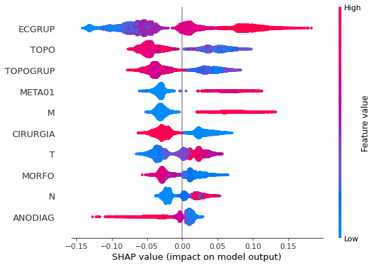
plot_feat_importances(xgb_sp_04_07, feat_SP_04_07)
Here we noticed that the most used feature was
ECGRUP, with a good advantage over the others. Following we haveREC01,CIRURGIAandIDADE.
[ ]:
plot_shap_values(xgb_sp_04_07, X_testSP_04_07, feat_SP_04_07)
Note that larger values of the ECGRUP column, shown in pink, have more influence for the model’s prediction to be class 1, smaller values have greater weight for the prediction to be class 0. This behavior was expected, because the higher the clinical stage, worse is the stage of cancer.
The other columns shown follow the same logic.
[ ]:
# SP - 2008 to 2011
xgb_sp_08_11 = XGBClassifier(max_depth=8,
                             scale_pos_weight=1.15,
                             random_state=seed)

xgb_sp_08_11.fit(X_trainSP_08_11, y_trainSP_08_11)
XGBClassifier(max_depth=8, random_state=10, scale_pos_weight=1.15)
[ ]:
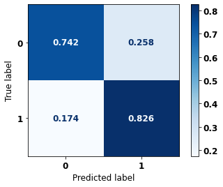
display_confusion_matrix(xgb_sp_08_11, X_testSP_08_11, y_testSP_08_11)
              precision    recall  f1-score   support

           0      0.814     0.817     0.816     13681
           1      0.822     0.818     0.820     14062

    accuracy                          0.818     27743
   macro avg      0.818     0.818     0.818     27743
weighted avg      0.818     0.818     0.818     27743
The confusion matrix obtained for the XGBoost, with SP data from 2008 to 2011, shows a good performance of the model, with 82% of accuracy.
[ ]:
plot_roc_curve(xgb_sp_08_11, X_trainSP_08_11, X_testSP_08_11, y_trainSP_08_11, y_testSP_08_11)
[ ]:
plot_feat_importances(xgb_sp_08_11, feat_SP_08_11)
Here we noticed that the most used feature was
ECGRUP, with a good advantage over the others. Following we haveREC01,CIRURGIAandRECNENHUM.
[ ]:
plot_shap_values(xgb_sp_08_11, X_testSP_08_11, feat_SP_08_11)
Note that larger values of the ECGRUP column, shown in pink, have more influence for the model’s prediction to be class 1, smaller values have greater weight for the prediction to be class 0. This behavior was expected, because the higher the clinical stage, worse is the stage of cancer.
The other columns shown follow the same logic.
[ ]:
# SP - 2012 to 2015
xgb_sp_12_15 = XGBClassifier(max_depth=8,
                             random_state=seed,
                             scale_pos_weight=1.79)

xgb_sp_12_15.fit(X_trainSP_12_15, y_trainSP_12_15)
XGBClassifier(max_depth=8, random_state=10, scale_pos_weight=1.79)
[ ]:
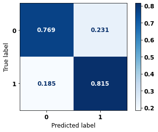
display_confusion_matrix(xgb_sp_12_15, X_testSP_12_15, y_testSP_12_15)

              precision    recall  f1-score   support

           0      0.887     0.829     0.857     21356
           1      0.750     0.829     0.788     13274

    accuracy                          0.829     34630
   macro avg      0.818     0.829     0.822     34630
weighted avg      0.834     0.829     0.830     34630
The confusion matrix obtained for the XGBoost, with SP data from 2012 to 2015, shows a good performance of the model, with 83% of accuracy.
[ ]:
plot_roc_curve(xgb_sp_12_15, X_trainSP_12_15, X_testSP_12_15, y_trainSP_12_15, y_testSP_12_15)

[ ]:
plot_feat_importances(xgb_sp_12_15, feat_SP_12_15)
Here we noticed that the most used feature was
ECGRUP, with a good advantage. Following we haveRECNENHUM,REC01andCIRURGIA.
[ ]:
plot_shap_values(xgb_sp_12_15, X_testSP_12_15, feat_SP_12_15)
Note that larger values of the ECGRUP column, shown in pink, have more influence for the model’s prediction to be class 1, smaller values have greater weight for the prediction to be class 0. This behavior was expected, because the higher the clinical stage, worse is the stage of cancer.
The other columns shown follow the same logic.
[ ]:
# SP - 2016 to 2021
xgb_sp_16_21 = XGBClassifier(max_depth=8,
                             random_state=seed,
                             scale_pos_weight=3)

xgb_sp_16_21.fit(X_trainSP_16_21, y_trainSP_16_21)
XGBClassifier(max_depth=8, random_state=10, scale_pos_weight=3)
[ ]:
display_confusion_matrix(xgb_sp_16_21, X_testSP_16_21, y_testSP_16_21)

              precision    recall  f1-score   support

           0      0.930     0.830     0.877     19497
           1      0.641     0.829     0.723      7129

    accuracy                          0.830     26626
   macro avg      0.785     0.829     0.800     26626
weighted avg      0.852     0.830     0.836     26626
The confusion matrix obtained for the XGBoost, with SP data from 2016 to 2021, shows a good performance of the model, with 83% of accuracy.
[ ]:
plot_roc_curve(xgb_sp_16_21, X_trainSP_16_21, X_testSP_16_21, y_trainSP_16_21, y_testSP_16_21)

[ ]:
plot_feat_importances(xgb_sp_16_21, feat_SP_16_21)
The four most important features were
ECGRUP,RECDIST,RECNENHUMandGLEASON.
[ ]:
plot_shap_values(xgb_sp_16_21, X_testSP_16_21, feat_SP_16_21)
Note that larger values of the ECGRUP column, shown in pink, have more influence for the model’s prediction to be class 1, smaller values have greater weight for the prediction to be class 0. This behavior was expected, because the higher the clinical stage, worse is the stage of cancer.
The other columns shown follow the same logic.
Other states
[ ]:
# Other states - 2000 to 2003
xgb_fora_00_03 = XGBClassifier(max_depth=5,
                               scale_pos_weight=0.705,
                               random_state=seed)

xgb_fora_00_03.fit(X_trainOS_00_03, y_trainOS_00_03)
XGBClassifier(max_depth=5, random_state=10, scale_pos_weight=0.705)
[ ]:
display_confusion_matrix(xgb_fora_00_03, X_testOS_00_03, y_testOS_00_03)

              precision    recall  f1-score   support

           0      0.695     0.755     0.724       396
           1      0.808     0.757     0.782       539

    accuracy                          0.756       935
   macro avg      0.752     0.756     0.753       935
weighted avg      0.760     0.756     0.757       935
The confusion matrix obtained for the XGBoost, with other states data from 2000 to 2003, also shows a good performance of the model, with 76% of accuracy.
[ ]:
plot_roc_curve(xgb_fora_00_03, X_trainOS_00_03, X_testOS_00_03, y_trainOS_00_03, y_testOS_00_03)
[ ]:
plot_feat_importances(xgb_fora_00_03, feat_OS_00_03)
Again we noticed that the most used feature was
ECGRUP, with a good advantage. The following most important features wereREC01,IDADEandM.
[ ]:
plot_shap_values(xgb_fora_00_03, X_testOS_00_03, feat_OS_00_03)
Note that larger values of the ECGRUP column, shown in pink, have more influence for the model’s prediction to be class 1, smaller values have greater weight for the prediction to be class 0. This behavior was expected, because the higher the clinical stage, worse is the stage of cancer.
The other columns shown follow the same logic.
[ ]:
# Other states - 2004 to 2007
xgb_fora_04_07 = XGBClassifier(max_depth=5,
                               scale_pos_weight=1.13,
                               random_state=seed)

xgb_fora_04_07.fit(X_trainOS_04_07, y_trainOS_04_07)
XGBClassifier(max_depth=5, random_state=10, scale_pos_weight=1.13)
[ ]:
display_confusion_matrix(xgb_fora_04_07, X_testOS_04_07, y_testOS_04_07)
              precision    recall  f1-score   support

           0      0.801     0.791     0.796       678
           1      0.780     0.791     0.786       637

    accuracy                          0.791      1315
   macro avg      0.791     0.791     0.791      1315
weighted avg      0.791     0.791     0.791      1315
The confusion matrix obtained for the XGBoost, with other states data from 2004 to 2007, also shows a good performance of the model with 79% of accuracy.
[ ]:
plot_roc_curve(xgb_fora_04_07, X_trainOS_04_07, X_testOS_04_07, y_trainOS_04_07, y_testOS_04_07)
[ ]:
plot_feat_importances(xgb_fora_04_07, feat_OS_04_07)
Again we noticed that the most used feature was
ECGRUP, with a good advantage. The following most important features wereREC01,CIRURGIAandTOPO.
[ ]:
plot_shap_values(xgb_fora_04_07, X_testOS_04_07, feat_OS_04_07)
Note that larger values of the ECGRUP column, shown in pink, have more influence for the model’s prediction to be class 1, smaller values have greater weight for the prediction to be class 0. This behavior was expected, because the higher the clinical stage, worse is the stage of cancer.
The other columns shown follow the same logic.
[ ]:
# Other states - 2008 to 2011
xgb_fora_08_11 = XGBClassifier(max_depth=5,
                               scale_pos_weight=1.27,
                               random_state=seed)

xgb_fora_08_11.fit(X_trainOS_08_11, y_trainOS_08_11)
XGBClassifier(max_depth=5, random_state=10, scale_pos_weight=1.27)
[ ]:
display_confusion_matrix(xgb_fora_08_11, X_testOS_08_11, y_testOS_08_11)
              precision    recall  f1-score   support

           0      0.844     0.803     0.823       921
           1      0.754     0.802     0.778       693

    accuracy                          0.803      1614
   macro avg      0.799     0.803     0.800      1614
weighted avg      0.805     0.803     0.804      1614
The confusion matrix obtained for the XGBoost, with other states data from 2008 to 2011, also shows a good performance of the model with 80% of accuracy.
[ ]:
plot_roc_curve(xgb_fora_08_11, X_trainOS_08_11, X_testOS_08_11, y_trainOS_08_11, y_testOS_08_11)

[ ]:
plot_feat_importances(xgb_fora_08_11, feat_OS_08_11)
Again we noticed that the most used feature was
ECGRUP, with a lot advantage. The following most important features wereREC01,MandCIRURGIA.
[ ]:
plot_shap_values(xgb_fora_08_11, X_testOS_08_11, feat_OS_08_11)
Note that larger values of the ECGRUP column, shown in pink, have more influence for the model’s prediction to be class 1, smaller values have greater weight for the prediction to be class 0. This behavior was expected, because the higher the clinical stage, worse is the stage of cancer.
The other columns shown follow the same logic.
[ ]:
# Other states - 2012 to 2015
xgb_fora_12_15 = XGBClassifier(max_depth=5,
                               scale_pos_weight=2.835,
                               random_state=seed)

xgb_fora_12_15.fit(X_trainOS_12_15, y_trainOS_12_15)
XGBClassifier(max_depth=5, random_state=10, scale_pos_weight=2.835)
[ ]:
display_confusion_matrix(xgb_fora_12_15, X_testOS_12_15, y_testOS_12_15)

              precision    recall  f1-score   support

           0      0.896     0.804     0.848      1452
           1      0.665     0.806     0.729       701

    accuracy                          0.805      2153
   macro avg      0.781     0.805     0.788      2153
weighted avg      0.821     0.805     0.809      2153
The confusion matrix obtained for the XGBoost, with other states data from 2012 to 2015, also shows a good performance of the model with 80% of accuracy.
[ ]:
plot_roc_curve(xgb_fora_12_15, X_trainOS_12_15, X_testOS_12_15, y_trainOS_12_15, y_testOS_12_15)
[ ]:
plot_feat_importances(xgb_fora_12_15, feat_OS_12_15)
The four most important features were
ECGRUP,META01,REC01andPM.
[ ]:
plot_shap_values(xgb_fora_12_15, X_testOS_12_15, feat_OS_12_15)
Note that larger values of the ECGRUP column, shown in pink, have more influence for the model’s prediction to be class 1, smaller values have greater weight for the prediction to be class 0. This behavior was expected, because the higher the clinical stage, worse is the stage of cancer.
The other columns shown follow the same logic.
[ ]:
# Other states - 2016 to 2020
xgb_fora_16_20 = XGBClassifier(max_depth=5,
                               scale_pos_weight=3.2,
                               random_state=seed)

xgb_fora_16_20.fit(X_trainOS_16_20, y_trainOS_16_20)
XGBClassifier(max_depth=5, random_state=10, scale_pos_weight=3.2)
[ ]:
display_confusion_matrix(xgb_fora_16_20, X_testOS_16_20, y_testOS_16_20)
              precision    recall  f1-score   support

           0      0.932     0.823     0.874      1643
           1      0.616     0.825     0.706       565

    accuracy                          0.824      2208
   macro avg      0.774     0.824     0.790      2208
weighted avg      0.851     0.824     0.831      2208
The confusion matrix obtained for the XGBoost, with other states data from 2016 to 2020, shows the best performance comparing with the other models, with 82% of accuracy.
[ ]:
plot_roc_curve(xgb_fora_16_20, X_trainOS_16_20, X_testOS_16_20, y_trainOS_16_20, y_testOS_16_20)
[ ]:
plot_feat_importances(xgb_fora_16_20, feat_OS_16_20)
The four most important features were
ECGRUP,REC01,META01andCIRURGIA.
[ ]:
plot_shap_values(xgb_fora_16_20, X_testOS_16_20, feat_OS_16_20)
Note that larger values of the ECGRUP column, shown in pink, have more influence for the model’s prediction to be class 1, smaller values have greater weight for the prediction to be class 0. This behavior was expected, because the higher the clinical stage, worse is the stage of cancer.
The other columns shown follow the same logic.
Testing models with data from other years
We will use test data from the following years in the trained models for each set of years grouped together.
Random Forest SP for years 2000 to 2003
[ ]:
display_confusion_matrix(rf_sp_00_03, X_testSP_04_07, y_testSP_04_07)
              precision    recall  f1-score   support

           0      0.743     0.761     0.752      8851
           1      0.821     0.806     0.814     12036

    accuracy                          0.787     20887
   macro avg      0.782     0.784     0.783     20887
weighted avg      0.788     0.787     0.787     20887
[ ]:
display_confusion_matrix(rf_sp_00_03, X_testSP_08_11, y_testSP_08_11)

              precision    recall  f1-score   support

           0      0.809     0.751     0.779     13681
           1      0.773     0.828     0.800     14062

    accuracy                          0.790     27743
   macro avg      0.791     0.789     0.789     27743
weighted avg      0.791     0.790     0.789     27743
[ ]:
display_confusion_matrix(rf_sp_00_03, X_testSP_12_15, y_testSP_12_15)

              precision    recall  f1-score   support

           0      0.907     0.692     0.785     21356
           1      0.641     0.885     0.744     13274

    accuracy                          0.766     34630
   macro avg      0.774     0.789     0.765     34630
weighted avg      0.805     0.766     0.769     34630
[ ]:
display_confusion_matrix(rf_sp_00_03, X_testSP_16_21, y_testSP_16_21)
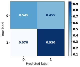
              precision    recall  f1-score   support

           0      0.955     0.545     0.694     19497
           1      0.428     0.930     0.586      7129

    accuracy                          0.649     26626
   macro avg      0.692     0.738     0.640     26626
weighted avg      0.814     0.649     0.665     26626
XGBoost SP for years 2000 to 2003
[ ]:
display_confusion_matrix(xgb_sp_00_03, X_testSP_04_07, y_testSP_04_07)
              precision    recall  f1-score   support

           0      0.754     0.769     0.761      8851
           1      0.828     0.815     0.821     12036

    accuracy                          0.796     20887
   macro avg      0.791     0.792     0.791     20887
weighted avg      0.796     0.796     0.796     20887
[ ]:
display_confusion_matrix(xgb_sp_00_03, X_testSP_08_11, y_testSP_08_11)
              precision    recall  f1-score   support

           0      0.805     0.742     0.772     13681
           1      0.767     0.826     0.795     14062

    accuracy                          0.784     27743
   macro avg      0.786     0.784     0.784     27743
weighted avg      0.786     0.784     0.784     27743
[ ]:
display_confusion_matrix(xgb_sp_00_03, X_testSP_12_15, y_testSP_12_15)
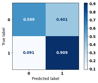
              precision    recall  f1-score   support

           0      0.914     0.599     0.724     21356
           1      0.585     0.909     0.712     13274

    accuracy                          0.718     34630
   macro avg      0.749     0.754     0.718     34630
weighted avg      0.788     0.718     0.719     34630
[ ]:
display_confusion_matrix(xgb_sp_00_03, X_testSP_16_21, y_testSP_16_21)

              precision    recall  f1-score   support

           0      0.964     0.293     0.449     19497
           1      0.334     0.970     0.497      7129

    accuracy                          0.474     26626
   macro avg      0.649     0.631     0.473     26626
weighted avg      0.795     0.474     0.462     26626
Random Forest SP for years 2004 to 2007
[ ]:
display_confusion_matrix(rf_sp_04_07, X_testSP_08_11, y_testSP_08_11)

              precision    recall  f1-score   support

           0      0.804     0.775     0.790     13681
           1      0.789     0.816     0.802     14062

    accuracy                          0.796     27743
   macro avg      0.797     0.796     0.796     27743
weighted avg      0.796     0.796     0.796     27743
[ ]:
display_confusion_matrix(rf_sp_04_07, X_testSP_12_15, y_testSP_12_15)
              precision    recall  f1-score   support

           0      0.913     0.691     0.787     21356
           1      0.643     0.894     0.748     13274

    accuracy                          0.769     34630
   macro avg      0.778     0.792     0.767     34630
weighted avg      0.809     0.769     0.772     34630
[ ]:
display_confusion_matrix(rf_sp_04_07, X_testSP_16_21, y_testSP_16_21)

              precision    recall  f1-score   support

           0      0.956     0.576     0.719     19497
           1      0.444     0.928     0.601      7129

    accuracy                          0.670     26626
   macro avg      0.700     0.752     0.660     26626
weighted avg      0.819     0.670     0.687     26626
XGBoost SP for years 2004 to 2007
[ ]:
display_confusion_matrix(xgb_sp_04_07, X_testSP_08_11, y_testSP_08_11)
              precision    recall  f1-score   support

           0      0.821     0.760     0.789     13681
           1      0.782     0.839     0.810     14062

    accuracy                          0.800     27743
   macro avg      0.802     0.799     0.799     27743
weighted avg      0.801     0.800     0.800     27743
[ ]:
display_confusion_matrix(xgb_sp_04_07, X_testSP_12_15, y_testSP_12_15)
              precision    recall  f1-score   support

           0      0.855     0.487     0.621     21356
           1      0.513     0.868     0.644     13274

    accuracy                          0.633     34630
   macro avg      0.684     0.677     0.633     34630
weighted avg      0.724     0.633     0.630     34630
[ ]:
display_confusion_matrix(xgb_sp_04_07, X_testSP_16_21, y_testSP_16_21)

              precision    recall  f1-score   support

           0      0.900     0.494     0.638     19497
           1      0.380     0.849     0.525      7129

    accuracy                          0.589     26626
   macro avg      0.640     0.672     0.582     26626
weighted avg      0.761     0.589     0.608     26626
Random Forest SP for years 2008 to 2011
[ ]:
display_confusion_matrix(rf_sp_08_11, X_testSP_12_15, y_testSP_12_15)

              precision    recall  f1-score   support

           0      0.896     0.754     0.819     21356
           1      0.685     0.860     0.762     13274

    accuracy                          0.794     34630
   macro avg      0.790     0.807     0.791     34630
weighted avg      0.815     0.794     0.797     34630
[ ]:
display_confusion_matrix(rf_sp_08_11, X_testSP_16_21, y_testSP_16_21)
              precision    recall  f1-score   support

           0      0.953     0.620     0.751     19497
           1      0.469     0.916     0.620      7129

    accuracy                          0.699     26626
   macro avg      0.711     0.768     0.686     26626
weighted avg      0.823     0.699     0.716     26626
XGBoost SP for years 2008 to 2011
[ ]:
display_confusion_matrix(xgb_sp_08_11, X_testSP_12_15, y_testSP_12_15)

              precision    recall  f1-score   support

           0      0.886     0.689     0.775     21356
           1      0.632     0.858     0.727     13274

    accuracy                          0.754     34630
   macro avg      0.759     0.773     0.751     34630
weighted avg      0.789     0.754     0.757     34630
[ ]:
display_confusion_matrix(xgb_sp_08_11, X_testSP_16_21, y_testSP_16_21)
              precision    recall  f1-score   support

           0      0.953     0.268     0.418     19497
           1      0.325     0.964     0.486      7129

    accuracy                          0.454     26626
   macro avg      0.639     0.616     0.452     26626
weighted avg      0.785     0.454     0.436     26626
Random Forest SP for years 2012 to 2015
[ ]:
display_confusion_matrix(rf_sp_12_15, X_testSP_16_21, y_testSP_16_21)

              precision    recall  f1-score   support

           0      0.933     0.723     0.815     19497
           1      0.531     0.857     0.656      7129

    accuracy                          0.759     26626
   macro avg      0.732     0.790     0.735     26626
weighted avg      0.825     0.759     0.772     26626
XGBoost SP for years 2012 to 2015
[ ]:
display_confusion_matrix(xgb_sp_12_15, X_testSP_16_21, y_testSP_16_21)

              precision    recall  f1-score   support

           0      0.938     0.736     0.825     19497
           1      0.546     0.867     0.670      7129

    accuracy                          0.771     26626
   macro avg      0.742     0.801     0.747     26626
weighted avg      0.833     0.771     0.783     26626
Random Forest Other states for years 2000 to 2003
[ ]:
display_confusion_matrix(rf_fora_00_03, X_testOS_04_07, y_testOS_04_07)

              precision    recall  f1-score   support

           0      0.808     0.740     0.773       678
           1      0.746     0.813     0.778       637

    accuracy                          0.776      1315
   macro avg      0.777     0.777     0.776      1315
weighted avg      0.778     0.776     0.776      1315
[ ]:
display_confusion_matrix(rf_fora_00_03, X_testOS_08_11, y_testOS_08_11)

              precision    recall  f1-score   support

           0      0.866     0.701     0.775       921
           1      0.683     0.856     0.760       693

    accuracy                          0.768      1614
   macro avg      0.775     0.779     0.767      1614
weighted avg      0.787     0.768     0.768      1614
[ ]:
display_confusion_matrix(rf_fora_00_03, X_testOS_12_15, y_testOS_12_15)
              precision    recall  f1-score   support

           0      0.909     0.670     0.772      1452
           1      0.558     0.862     0.677       701

    accuracy                          0.732      2153
   macro avg      0.734     0.766     0.724      2153
weighted avg      0.795     0.732     0.741      2153
[ ]:
display_confusion_matrix(rf_fora_00_03, X_testOS_16_20, y_testOS_16_20)
              precision    recall  f1-score   support

           0      0.962     0.611     0.747      1643
           1      0.451     0.929     0.607       565

    accuracy                          0.692      2208
   macro avg      0.706     0.770     0.677      2208
weighted avg      0.831     0.692     0.711      2208
XGBoost Other states for years 2000 to 2003
[ ]:
display_confusion_matrix(xgb_fora_00_03, X_testOS_04_07, y_testOS_04_07)
              precision    recall  f1-score   support

           0      0.789     0.770     0.779       678
           1      0.761     0.780     0.771       637

    accuracy                          0.775      1315
   macro avg      0.775     0.775     0.775      1315
weighted avg      0.775     0.775     0.775      1315
[ ]:
display_confusion_matrix(xgb_fora_00_03, X_testOS_08_11, y_testOS_08_11)
              precision    recall  f1-score   support

           0      0.852     0.744     0.794       921
           1      0.709     0.828     0.764       693

    accuracy                          0.780      1614
   macro avg      0.780     0.786     0.779      1614
weighted avg      0.790     0.780     0.781      1614
[ ]:
display_confusion_matrix(xgb_fora_00_03, X_testOS_12_15, y_testOS_12_15)

              precision    recall  f1-score   support

           0      0.895     0.719     0.798      1452
           1      0.587     0.826     0.686       701

    accuracy                          0.754      2153
   macro avg      0.741     0.772     0.742      2153
weighted avg      0.795     0.754     0.761      2153
[ ]:
display_confusion_matrix(xgb_fora_00_03, X_testOS_16_20, y_testOS_16_20)

              precision    recall  f1-score   support

           0      0.950     0.677     0.791      1643
           1      0.488     0.896     0.632       565

    accuracy                          0.733      2208
   macro avg      0.719     0.786     0.711      2208
weighted avg      0.832     0.733     0.750      2208
Random Forest Other states for years 2004 to 2007
[ ]:
display_confusion_matrix(rf_fora_04_07, X_testOS_08_11, y_testOS_08_11)
              precision    recall  f1-score   support

           0      0.849     0.744     0.793       921
           1      0.708     0.824     0.761       693

    accuracy                          0.778      1614
   macro avg      0.778     0.784     0.777      1614
weighted avg      0.788     0.778     0.779      1614
[ ]:
display_confusion_matrix(rf_fora_04_07, X_testOS_12_15, y_testOS_12_15)

              precision    recall  f1-score   support

           0      0.903     0.709     0.794      1452
           1      0.583     0.843     0.689       701

    accuracy                          0.752      2153
   macro avg      0.743     0.776     0.742      2153
weighted avg      0.799     0.752     0.760      2153
[ ]:
display_confusion_matrix(rf_fora_04_07, X_testOS_16_20, y_testOS_16_20)
              precision    recall  f1-score   support

           0      0.963     0.632     0.763      1643
           1      0.465     0.929     0.620       565

    accuracy                          0.708      2208
   macro avg      0.714     0.781     0.692      2208
weighted avg      0.836     0.708     0.727      2208
XGBoost Other states for years 2004 to 2007
[ ]:
display_confusion_matrix(xgb_fora_04_07, X_testOS_08_11, y_testOS_08_11)

              precision    recall  f1-score   support

           0      0.876     0.738     0.801       921
           1      0.712     0.861     0.780       693

    accuracy                          0.791      1614
   macro avg      0.794     0.800     0.791      1614
weighted avg      0.806     0.791     0.792      1614
[ ]:
display_confusion_matrix(xgb_fora_04_07, X_testOS_12_15, y_testOS_12_15)

              precision    recall  f1-score   support

           0      0.909     0.701     0.792      1452
           1      0.580     0.854     0.691       701

    accuracy                          0.751      2153
   macro avg      0.744     0.778     0.741      2153
weighted avg      0.802     0.751     0.759      2153
[ ]:
display_confusion_matrix(xgb_fora_04_07, X_testOS_16_20, y_testOS_16_20)
              precision    recall  f1-score   support

           0      0.964     0.632     0.764      1643
           1      0.465     0.931     0.621       565

    accuracy                          0.709      2208
   macro avg      0.715     0.782     0.692      2208
weighted avg      0.836     0.709     0.727      2208
Random Forest Other states for years 2008 to 2011
[ ]:
display_confusion_matrix(rf_fora_08_11, X_testOS_12_15, y_testOS_12_15)

              precision    recall  f1-score   support

           0      0.900     0.764     0.827      1452
           1      0.628     0.823     0.712       701

    accuracy                          0.784      2153
   macro avg      0.764     0.794     0.769      2153
weighted avg      0.811     0.784     0.789      2153
[ ]:
display_confusion_matrix(rf_fora_08_11, X_testOS_16_20, y_testOS_16_20)

              precision    recall  f1-score   support

           0      0.947     0.691     0.799      1643
           1      0.497     0.887     0.637       565

    accuracy                          0.741      2208
   macro avg      0.722     0.789     0.718      2208
weighted avg      0.832     0.741     0.758      2208
XGBoost Other states for years 2008 to 2011
[ ]:
display_confusion_matrix(xgb_fora_08_11, X_testOS_12_15, y_testOS_12_15)
              precision    recall  f1-score   support

           0      0.895     0.768     0.827      1452
           1      0.628     0.813     0.709       701

    accuracy                          0.783      2153
   macro avg      0.762     0.791     0.768      2153
weighted avg      0.808     0.783     0.788      2153
[ ]:
display_confusion_matrix(xgb_fora_08_11, X_testOS_16_20, y_testOS_16_20)

              precision    recall  f1-score   support

           0      0.949     0.710     0.812      1643
           1      0.513     0.888     0.650       565

    accuracy                          0.755      2208
   macro avg      0.731     0.799     0.731      2208
weighted avg      0.837     0.755     0.771      2208
Random Forest Other states for years 2012 to 2015
[ ]:
display_confusion_matrix(rf_fora_12_15, X_testOS_16_20, y_testOS_16_20)

              precision    recall  f1-score   support

           0      0.945     0.716     0.814      1643
           1      0.515     0.878     0.649       565

    accuracy                          0.757      2208
   macro avg      0.730     0.797     0.732      2208
weighted avg      0.835     0.757     0.772      2208
XGBoost Other states for years 2012 to 2015
[ ]:
display_confusion_matrix(xgb_fora_12_15, X_testOS_16_20, y_testOS_16_20)
              precision    recall  f1-score   support

           0      0.955     0.710     0.815      1643
           1      0.517     0.903     0.658       565

    accuracy                          0.760      2208
   macro avg      0.736     0.806     0.736      2208
weighted avg      0.843     0.760     0.774      2208
Fourth approach
Approach with grouped years, using only morphologies with final digit equal to 3 and without the column EC.
Preprocessing
Now we are going to divide the data into training and testing, and then do the preprocessing in both datasets to perform the training of the models and their evaluation. We will use the years grouped too, resulting in 5 datasets for SP and more 5 for other states.
First, it is necessary to define the columns that will be used as features and the label. We will not use some columns of the data: UFRESID, because we already have the division between SP and other states in the two datasets.
It was chosen to keep the column IDADE, so we will not use the FAIXAETAR, as well as the column ECGRUP and not the column EC. Finally, the other columns contained in the list list_drop are possible labels, so they will not be used as features for machine learning models.
[ ]:
list_drop = ['UFRESID', 'FAIXAETAR', 'ULTICONS', 'ULTIDIAG', 'ULTITRAT',
             'vivo_ano1', 'vivo_ano3', 'vivo_ano5', 'ULTINFO', 'EC', 'obito_cancer']

lb = 'obito_geral'
A function was created to perform the preprocessing, preprocessing, that uses the other functions created, get_train_test (divides the dataset into train and test sets), train_preprocessing (do the preprocessing of the train set) and test_preprocessing (do the preprocessing of the test set).
The process will be done 5 times for SP and other states, using the datasets with grouped years.
To see the complete function go to the functions section.
SP
[ ]:
X_trainSP_00_03, X_testSP_00_03, y_trainSP_00_03, y_testSP_00_03, feat_SP_00_03 = preprocessing(df_SP, list_drop, lb,
                                                                                                group_years=True, first_year=2000,
                                                                                                last_year=2003, morpho3=True,
                                                                                                random_state=seed,
                                                                                                balance_data=False,
                                                                                                encoder_type='LabelEncoder',
                                                                                                norm_name='StandardScaler')
X_train = (46098, 65), X_test = (15367, 65)
y_train = (46098,), y_test = (15367,)
[ ]:
X_trainSP_04_07, X_testSP_04_07, y_trainSP_04_07, y_testSP_04_07, feat_SP_04_07 = preprocessing(df_SP, list_drop, lb,
                                                                                                group_years=True, first_year=2004,
                                                                                                last_year=2007, morpho3=True,
                                                                                                random_state=seed,
                                                                                                balance_data=False,
                                                                                                encoder_type='LabelEncoder',
                                                                                                norm_name='StandardScaler')
X_train = (58169, 65), X_test = (19390, 65)
y_train = (58169,), y_test = (19390,)
[ ]:
X_trainSP_08_11, X_testSP_08_11, y_trainSP_08_11, y_testSP_08_11, feat_SP_08_11 = preprocessing(df_SP, list_drop, lb,
                                                                                                group_years=True, first_year=2008,
                                                                                                last_year=2011, morpho3=True,
                                                                                                random_state=seed,
                                                                                                balance_data=False,
                                                                                                encoder_type='LabelEncoder',
                                                                                                norm_name='StandardScaler')
X_train = (77412, 65), X_test = (25804, 65)
y_train = (77412,), y_test = (25804,)
[ ]:
X_trainSP_12_15, X_testSP_12_15, y_trainSP_12_15, y_testSP_12_15, feat_SP_12_15 = preprocessing(df_SP, list_drop, lb,
                                                                                                group_years=True, first_year=2012,
                                                                                                last_year=2015, morpho3=True,
                                                                                                random_state=seed,
                                                                                                balance_data=False,
                                                                                                encoder_type='LabelEncoder',
                                                                                                norm_name='StandardScaler')
X_train = (96124, 65), X_test = (32042, 65)
y_train = (96124,), y_test = (32042,)
[ ]:
X_trainSP_16_21, X_testSP_16_21, y_trainSP_16_21, y_testSP_16_21, feat_SP_16_21 = preprocessing(df_SP, list_drop, lb,
                                                                                                group_years=True, first_year=2016,
                                                                                                last_year=2021, morpho3=True,
                                                                                                random_state=seed,
                                                                                                balance_data=False,
                                                                                                encoder_type='LabelEncoder',
                                                                                                norm_name='StandardScaler')
X_train = (73682, 65), X_test = (24561, 65)
y_train = (73682,), y_test = (24561,)
Other states
[ ]:
X_trainOS_00_03, X_testOS_00_03, y_trainOS_00_03, y_testOS_00_03, feat_OS_00_03 = preprocessing(df_fora, list_drop, lb,
                                                                                                group_years=True, first_year=2000,
                                                                                                last_year=2003, morpho3=True,
                                                                                                random_state=seed,
                                                                                                balance_data=False,
                                                                                                encoder_type='LabelEncoder',
                                                                                                norm_name='StandardScaler')
X_train = (2592, 65), X_test = (865, 65)
y_train = (2592,), y_test = (865,)
[ ]:
X_trainOS_04_07, X_testOS_04_07, y_trainOS_04_07, y_testOS_04_07, feat_OS_04_07 = preprocessing(df_fora, list_drop, lb,
                                                                                                group_years=True, first_year=2004,
                                                                                                last_year=2007, morpho3=True,
                                                                                                random_state=seed,
                                                                                                balance_data=False,
                                                                                                encoder_type='LabelEncoder',
                                                                                                norm_name='StandardScaler')
X_train = (3694, 65), X_test = (1232, 65)
y_train = (3694,), y_test = (1232,)
[ ]:
X_trainOS_08_11, X_testOS_08_11, y_trainOS_08_11, y_testOS_08_11, feat_OS_08_11 = preprocessing(df_fora, list_drop, lb,
                                                                                                group_years=True, first_year=2008,
                                                                                                last_year=2011, morpho3=True,
                                                                                                random_state=seed,
                                                                                                balance_data=False,
                                                                                                encoder_type='LabelEncoder',
                                                                                                norm_name='StandardScaler')
X_train = (4536, 65), X_test = (1513, 65)
y_train = (4536,), y_test = (1513,)
[ ]:
X_trainOS_12_15, X_testOS_12_15, y_trainOS_12_15, y_testOS_12_15, feat_OS_12_15 = preprocessing(df_fora, list_drop, lb,
                                                                                                group_years=True, first_year=2012,
                                                                                                last_year=2015, morpho3=True,
                                                                                                random_state=seed,
                                                                                                balance_data=False,
                                                                                                encoder_type='LabelEncoder',
                                                                                                norm_name='StandardScaler')
X_train = (6069, 65), X_test = (2024, 65)
y_train = (6069,), y_test = (2024,)
[ ]:
X_trainOS_16_20, X_testOS_16_20, y_trainOS_16_20, y_testOS_16_20, feat_OS_16_20 = preprocessing(df_fora, list_drop, lb,
                                                                                                group_years=True, first_year=2016,
                                                                                                last_year=2020, morpho3=True,
                                                                                                random_state=seed,
                                                                                                balance_data=False,
                                                                                                encoder_type='LabelEncoder',
                                                                                                norm_name='StandardScaler')
X_train = (6185, 65), X_test = (2062, 65)
y_train = (6185,), y_test = (2062,)
Training and evaluation of the models
After dividing the data into training and testing, using the encoder and normalizing, the data is ready to be used by the machine learning models.
Random Forest
The first model is the Random Forest, the random_state will be used as a parameter, to obtain the same training values of the model every time it is runned.
The hyperparameter class_weight was used because the models have difficulty to learn the class with fewer examples.
SP
[ ]:
# SP - 2000 to 2003
rf_sp_00_03 = RandomForestClassifier(random_state=seed,
                                     class_weight={0:2.156, 1:1},
                                     criterion='entropy',
                                     max_depth=10)

rf_sp_00_03.fit(X_trainSP_00_03, y_trainSP_00_03)
RandomForestClassifier(class_weight={0: 2.156, 1: 1}, criterion='entropy',
                       max_depth=10, random_state=10)
[ ]:
display_confusion_matrix(rf_sp_00_03, X_testSP_00_03, y_testSP_00_03)

              precision    recall  f1-score   support

           0      0.607     0.773     0.680      4788
           1      0.883     0.774     0.825     10579

    accuracy                          0.774     15367
   macro avg      0.745     0.773     0.752     15367
weighted avg      0.797     0.774     0.780     15367
The confusion matrix obtained for the Random Forest, with SP data from 2000 to 2003, shows a good performance of the model, with 77% of accuracy.
[ ]:
show_tree(rf_sp_00_03, feat_SP_00_03, 2)
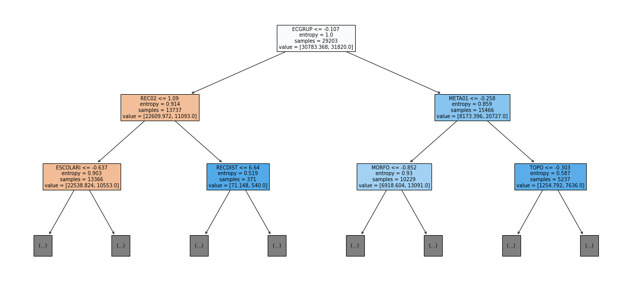
[ ]:
plot_roc_curve(rf_sp_00_03, X_trainSP_00_03, X_testSP_00_03, y_trainSP_00_03, y_testSP_00_03)
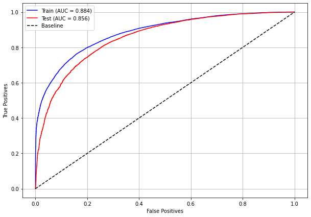
[ ]:
plot_feat_importances(rf_sp_00_03, feat_SP_00_03)
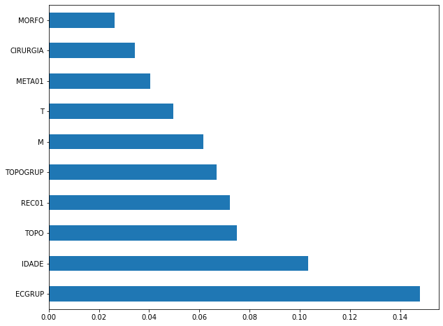
The four most important features in the model were
ECGRUP,IDADE,TOPO, andREC01.
[ ]:
plot_shap_values(rf_sp_00_03, X_testSP_00_03, feat_SP_00_03)
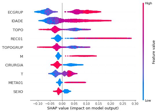
Note that larger values of the ECGRUP column, shown in pink, have more influence for the model’s prediction to be class 1, smaller values have greater weight for the prediction to be class 0. This behavior was expected, because the higher the clinical stage, worse is the stage of cancer.
The other columns shown follow the same logic.
[ ]:
# SP - 2004 to 2007
rf_sp_04_07 = RandomForestClassifier(random_state=seed,
                                     class_weight={0:1.28, 1:1},
                                     criterion='entropy',
                                     max_depth=10)

rf_sp_04_07.fit(X_trainSP_04_07, y_trainSP_04_07)
RandomForestClassifier(class_weight={0: 1.28, 1: 1}, criterion='entropy',
max_depth=10, random_state=10)
[ ]:
display_confusion_matrix(rf_sp_04_07, X_testSP_04_07, y_testSP_04_07)

precision recall f1-score support
0 0.693 0.778 0.733 7582
1 0.845 0.779 0.811 11808
accuracy 0.778 19390
macro avg 0.769 0.778 0.772 19390
weighted avg 0.786 0.778 0.780 19390
The confusion matrix obtained for the Random Forest, with SP data from 2004 to 2007, shows a good performance of the model, with 78% of accuracy.
[ ]:
show_tree(rf_sp_04_07, feat_SP_04_07, 2)
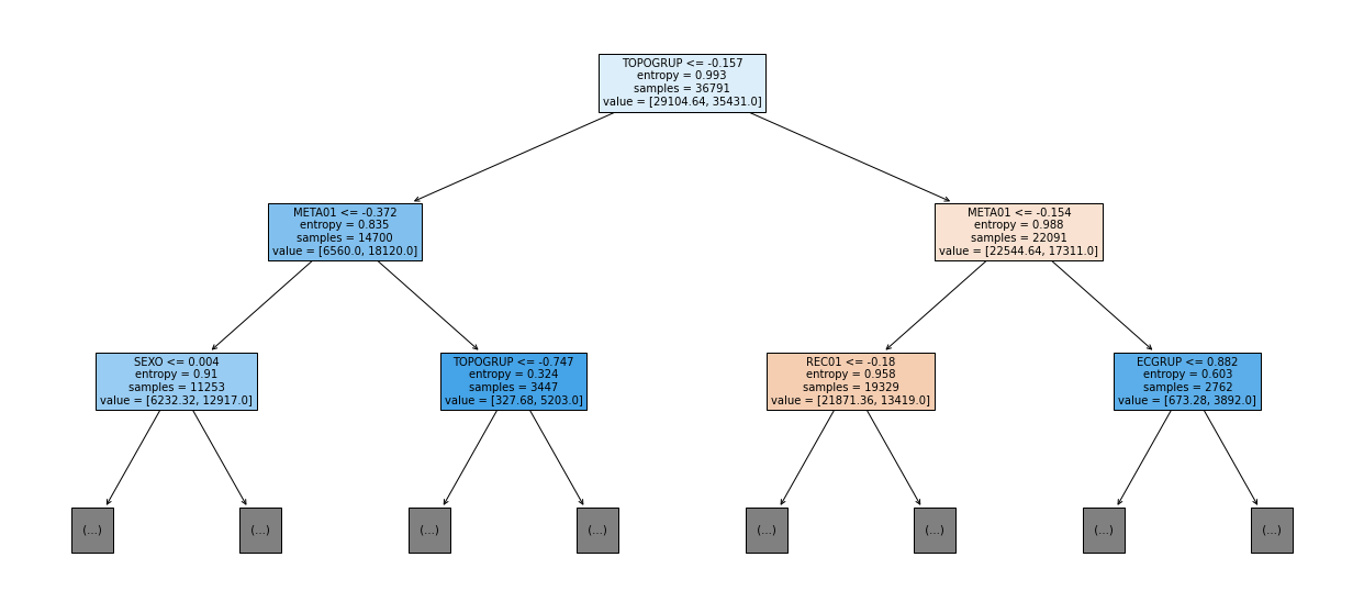
[ ]:
plot_roc_curve(rf_sp_04_07, X_trainSP_04_07, X_testSP_04_07, y_trainSP_04_07, y_testSP_04_07)
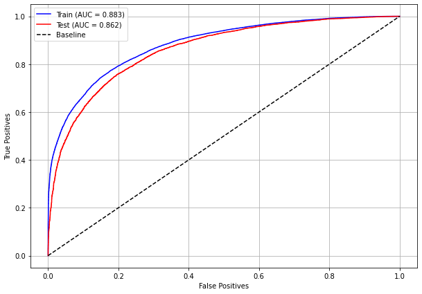
[ ]:
plot_feat_importances(rf_sp_04_07, feat_SP_04_07)
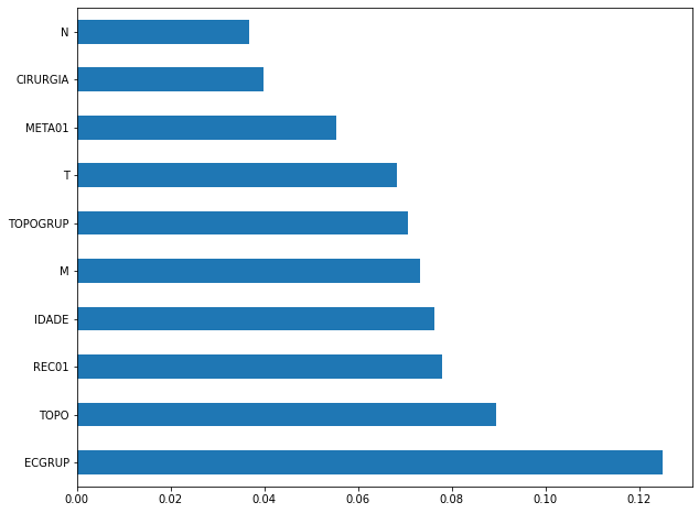
The four most important features in the model were
ECGRUP,TOPO,REC01andIDADE.
[ ]:
plot_shap_values(rf_sp_04_07, X_testSP_04_07, feat_SP_04_07)
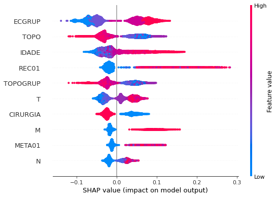
Note that larger values of the ECGRUP column, shown in pink, have more influence for the model’s prediction to be class 1, smaller values have greater weight for the prediction to be class 0. This behavior was expected, because the higher the clinical stage, worse is the stage of cancer.
The other columns shown follow the same logic.
[ ]:
# SP - 2008 to 2011
rf_sp_08_11 = RandomForestClassifier(random_state=seed,
class_weight={0:1, 1:1.0655},
criterion='entropy',
max_depth=10)
rf_sp_08_11.fit(X_trainSP_08_11, y_trainSP_08_11)
RandomForestClassifier(class_weight={0: 1, 1: 1.0655}, criterion='entropy',
max_depth=10, random_state=10)
[ ]:
display_confusion_matrix(rf_sp_08_11, X_testSP_08_11, y_testSP_08_11)

precision recall f1-score support
0 0.774 0.795 0.784 12014
1 0.817 0.797 0.807 13790
accuracy 0.796 25804
macro avg 0.795 0.796 0.795 25804
weighted avg 0.797 0.796 0.796 25804
The confusion matrix obtained for the Random Forest, with SP data from 2008 to 2011, shows a good performance of the model, with 80% of accuray.
[ ]:
show_tree(rf_sp_08_11, feat_SP_08_11, 2)

[ ]:
plot_roc_curve(rf_sp_08_11, X_trainSP_08_11, X_testSP_08_11, y_trainSP_08_11, y_testSP_08_11)
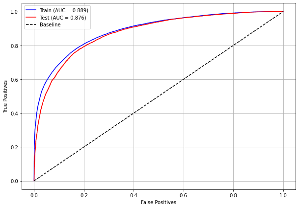
[ ]:
plot_feat_importances(rf_sp_08_11, feat_SP_08_11)
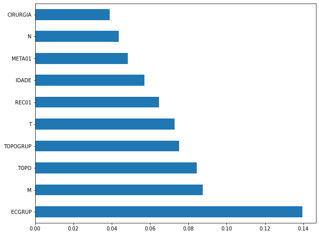
The four most important features in the model were
ECGRUP,M,TOPOandTOPOGRUP.
[ ]:
plot_shap_values(rf_sp_08_11, X_testSP_08_11, feat_SP_08_11)
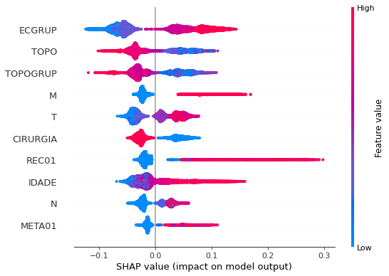
Note that larger values of the ECGRUP column, shown in pink, have more influence for the model’s prediction to be class 1, smaller values have greater weight for the prediction to be class 0. This behavior was expected, because the higher the clinical stage, worse is the stage of cancer.
The other columns shown follow the same logic.
[ ]:
# SP - 2012 to 2015
rf_sp_12_15 = RandomForestClassifier(random_state=seed,
class_weight={0:1, 1:1.778},
criterion='entropy',
max_depth=10)
rf_sp_12_15.fit(X_trainSP_12_15, y_trainSP_12_15)
RandomForestClassifier(class_weight={0: 1, 1: 1.778}, criterion='entropy',
max_depth=10, random_state=10)
[ ]:
display_confusion_matrix(rf_sp_12_15, X_testSP_12_15, y_testSP_12_15)

precision recall f1-score support
0 0.854 0.802 0.827 18944
1 0.737 0.802 0.768 13098
accuracy 0.802 32042
macro avg 0.795 0.802 0.798 32042
weighted avg 0.806 0.802 0.803 32042
The confusion matrix obtained for the Random Forest, with SP data from 2012 to 2015, shows a good performance of the model with 80% of accuracy.
[ ]:
show_tree(rf_sp_12_15, feat_SP_12_15, 2)
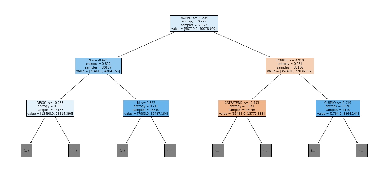
[ ]:
plot_roc_curve(rf_sp_12_15, X_trainSP_12_15, X_testSP_12_15, y_trainSP_12_15, y_testSP_12_15)
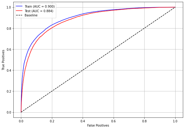
[ ]:
plot_feat_importances(rf_sp_12_15, feat_SP_12_15)
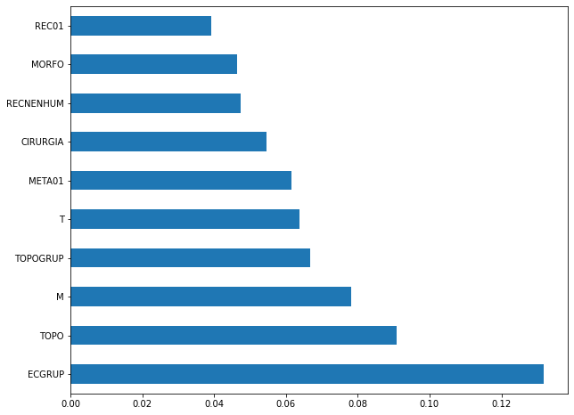
The four most important features in the model were
ECGRUP,TOPO,MandTOPOGRUP.
[ ]:
plot_shap_values(rf_sp_12_15, X_testSP_12_15, feat_SP_12_15)
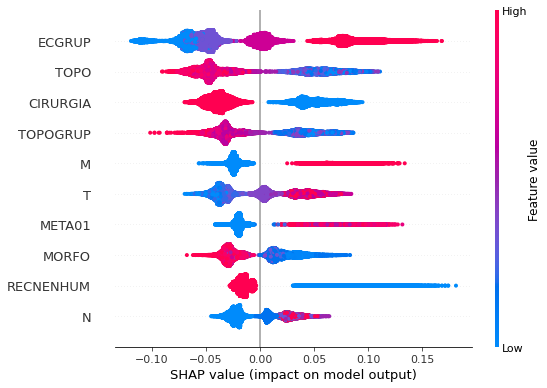
Note that larger values of the ECGRUP column, shown in pink, have more influence for the model’s prediction to be class 1, smaller values have greater weight for the prediction to be class 0. This behavior was expected, because the higher the clinical stage, worse is the stage of cancer.
The other columns shown follow the same logic.
[ ]:
# SP - 2016 to 2021
rf_sp_16_21 = RandomForestClassifier(random_state=seed,
class_weight={0:1, 1:2.58},
criterion='entropy',
max_depth=10)
rf_sp_16_21.fit(X_trainSP_16_21, y_trainSP_16_21)
RandomForestClassifier(class_weight={0: 1, 1: 2.58}, criterion='entropy',
max_depth=10, random_state=10)
[ ]:
display_confusion_matrix(rf_sp_16_21, X_testSP_16_21, y_testSP_16_21)
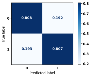
precision recall f1-score support
0 0.912 0.808 0.857 17508
1 0.628 0.807 0.707 7053
accuracy 0.808 24561
macro avg 0.770 0.808 0.782 24561
weighted avg 0.831 0.808 0.814 24561
The confusion matrix obtained for the Random Forest, with SP data from 2016 to 2021, shows a good performance of the model, with 81% of accuracy.
[ ]:
show_tree(rf_sp_16_21, feat_SP_16_21, 2)
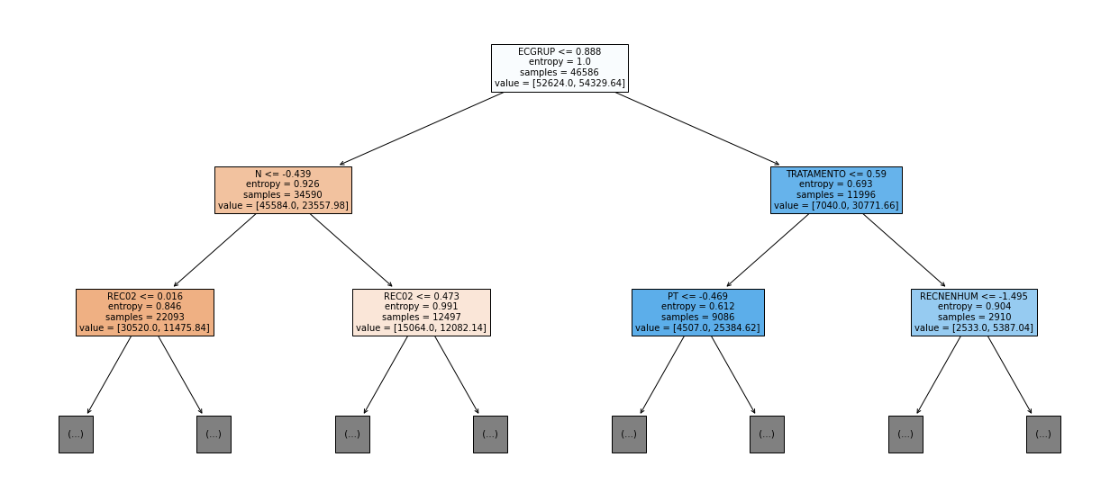
[ ]:
plot_roc_curve(rf_sp_16_21, X_trainSP_16_21, X_testSP_16_21, y_trainSP_16_21, y_testSP_16_21)
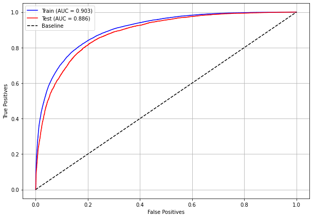
[ ]:
plot_feat_importances(rf_sp_16_21, feat_SP_16_21)
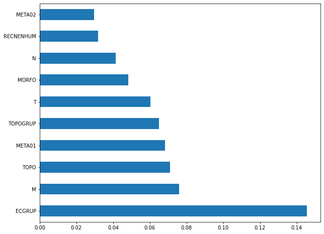
The four most important features in the model were
ECGRUP,M,TOPO, andMETA01.
[ ]:
plot_shap_values(rf_sp_16_21, X_testSP_16_21, feat_SP_16_21)
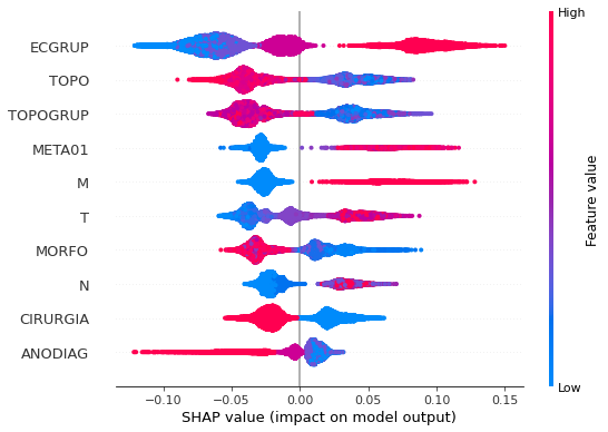
Note that larger values of the ECGRUP column, shown in pink, have more influence for the model’s prediction to be class 1, smaller values have greater weight for the prediction to be class 0. This behavior was expected, because the higher the clinical stage, worse is the stage of cancer.
The other columns shown follow the same logic.
Other states
[ ]:
# Other states - 2000 to 2003
rf_fora_00_03 = RandomForestClassifier(random_state=seed,
class_weight={0:1.285, 1:1},
criterion='entropy',
max_depth=6)
rf_fora_00_03.fit(X_trainOS_00_03, y_trainOS_00_03)
RandomForestClassifier(class_weight={0: 1.285, 1: 1}, criterion='entropy',
max_depth=6, random_state=10)
[ ]:
display_confusion_matrix(rf_fora_00_03, X_testOS_00_03, y_testOS_00_03)
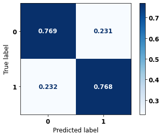
precision recall f1-score support
0 0.676 0.769 0.720 334
1 0.841 0.768 0.803 531
accuracy 0.769 865
macro avg 0.759 0.769 0.762 865
weighted avg 0.778 0.769 0.771 865
The confusion matrix obtained for the Random Forest, with other states data from 2000 to 2003, also shows a good performance of the model, and we have a balanced main diagonal with 77% of accuracy.
[ ]:
show_tree(rf_fora_00_03, feat_OS_00_03, 2)
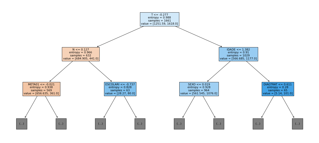
[ ]:
plot_roc_curve(rf_fora_00_03, X_trainOS_00_03, X_testOS_00_03, y_trainOS_00_03, y_testOS_00_03)
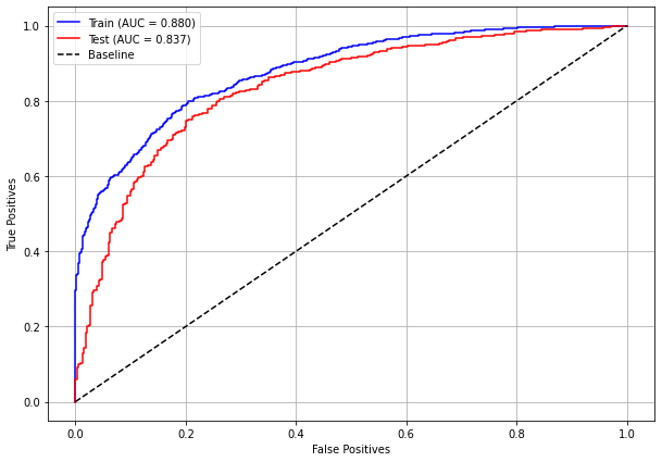
[ ]:
plot_feat_importances(rf_fora_00_03, feat_OS_00_03)
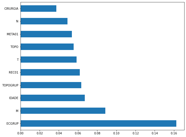
The four most important features in the model were
ECGRUP,M,IDADEandTOPOGRUP.
[ ]:
plot_shap_values(rf_fora_00_03, X_testOS_00_03, feat_OS_00_03)
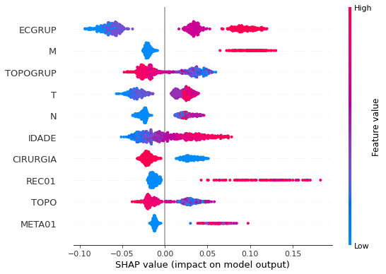
Note that larger values of the ECGRUP column, shown in pink, have more influence for the model’s prediction to be class 1, smaller values have greater weight for the prediction to be class 0. This behavior was expected, because the higher the clinical stage, worse is the stage of cancer.
The other columns shown follow the same logic.
[ ]:
# Other states - 2004 to 2007
rf_fora_04_07 = RandomForestClassifier(random_state=seed,
class_weight={0:1, 1:1.174},
criterion='entropy',
max_depth=6)
rf_fora_04_07.fit(X_trainOS_04_07, y_trainOS_04_07)
RandomForestClassifier(class_weight={0: 1, 1: 1.174}, criterion='entropy',
max_depth=6, random_state=10)
[ ]:
display_confusion_matrix(rf_fora_04_07, X_testOS_04_07, y_testOS_04_07)

precision recall f1-score support
0 0.757 0.765 0.761 600
1 0.775 0.767 0.771 632
accuracy 0.766 1232
macro avg 0.766 0.766 0.766 1232
weighted avg 0.766 0.766 0.766 1232
The confusion matrix obtained for the Random Forest, with other states data from 2004 to 2007, also shows a good performance of the model, with 77% of accuracy.
[ ]:
show_tree(rf_fora_04_07, feat_OS_04_07, 2)
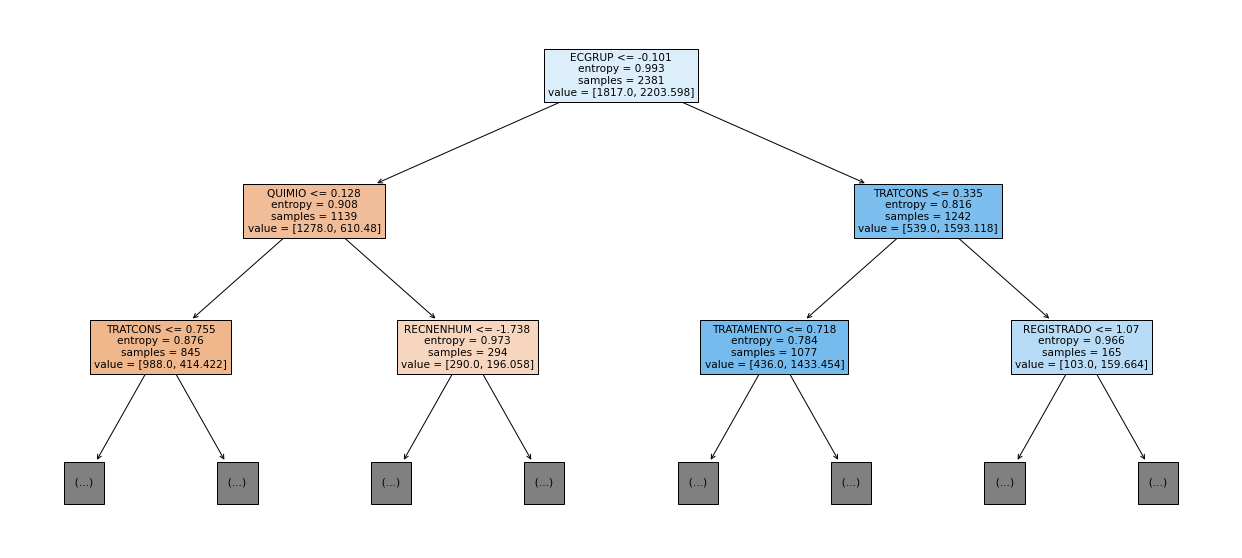
[ ]:
plot_roc_curve(rf_fora_04_07, X_trainOS_04_07, X_testOS_04_07, y_trainOS_04_07, y_testOS_04_07)

[ ]:
plot_feat_importances(rf_fora_04_07, feat_OS_04_07)
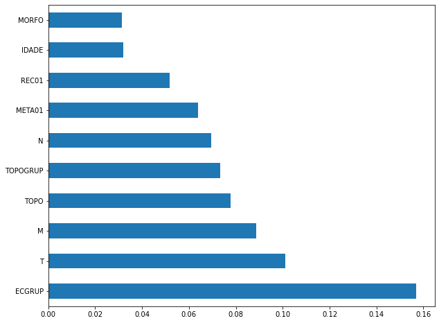
The four most important features in the model were
ECGRUP,T,MandTOPO.
[ ]:
plot_shap_values(rf_fora_04_07, X_testOS_04_07, feat_OS_04_07)
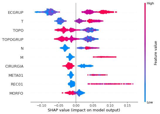
Note that larger values of the ECGRUP column, shown in pink, have more influence for the model’s prediction to be class 1, smaller values have greater weight for the prediction to be class 0. This behavior was expected, because the higher the clinical stage, worse is the stage of cancer.
The other columns shown follow the same logic.
[ ]:
# Other states - 2008 to 2011
rf_fora_08_11 = RandomForestClassifier(random_state=seed,
class_weight={0:1, 1:1.3},
criterion='entropy',
max_depth=6)
rf_fora_08_11.fit(X_trainOS_08_11, y_trainOS_08_11)
RandomForestClassifier(class_weight={0: 1, 1: 1.3}, criterion='entropy',
max_depth=6, random_state=10)
[ ]:
display_confusion_matrix(rf_fora_08_11, X_testOS_08_11, y_testOS_08_11)

precision recall f1-score support
0 0.831 0.802 0.816 827
1 0.771 0.803 0.787 686
accuracy 0.802 1513
macro avg 0.801 0.802 0.801 1513
weighted avg 0.804 0.802 0.803 1513
The confusion matrix obtained for the Random Forest, with other states data from 2008 to 2011, also shows a good performance of the model, presenting 80% of accuracy.
[ ]:
show_tree(rf_fora_08_11, feat_OS_08_11, 2)
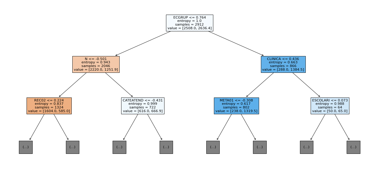
[ ]:
plot_roc_curve(rf_fora_08_11, X_trainOS_08_11, X_testOS_08_11, y_trainOS_08_11, y_testOS_08_11)
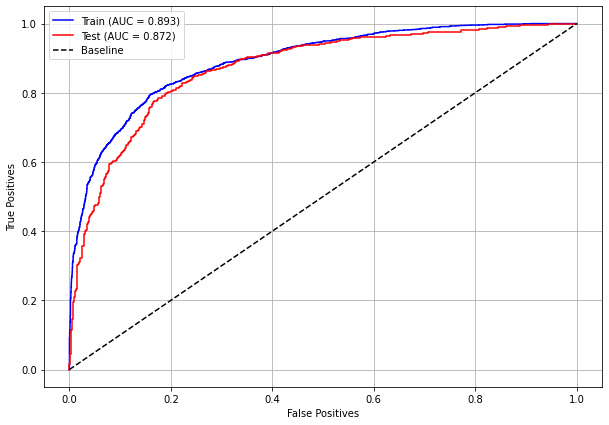
[ ]:
plot_feat_importances(rf_fora_08_11, feat_OS_08_11)
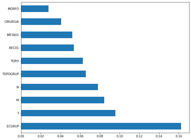
The four most important features in the model were
ECGRUP,T,MandN.
[ ]:
plot_shap_values(rf_fora_08_11, X_testOS_08_11, feat_OS_08_11)
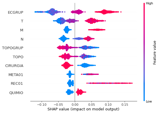
Note that larger values of the ECGRUP column, shown in pink, have more influence for the model’s prediction to be class 1, smaller values have greater weight for the prediction to be class 0. This behavior was expected, because the higher the clinical stage, worse is the stage of cancer.
The other columns shown follow the same logic.
[ ]:
# Other states - 2012 to 2015
rf_fora_12_15 = RandomForestClassifier(random_state=seed,
class_weight={0:1, 1:2.35},
criterion='entropy',
max_depth=6)
rf_fora_12_15.fit(X_trainOS_12_15, y_trainOS_12_15)
RandomForestClassifier(class_weight={0: 1, 1: 2.35}, criterion='entropy',
max_depth=6, random_state=10)
[ ]:
display_confusion_matrix(rf_fora_12_15, X_testOS_12_15, y_testOS_12_15)
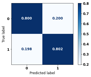
precision recall f1-score support
0 0.885 0.800 0.841 1327
1 0.678 0.802 0.735 697
accuracy 0.801 2024
macro avg 0.782 0.801 0.788 2024
weighted avg 0.814 0.801 0.804 2024
The confusion matrix obtained for the Random Forest, with other states data from 2012 to 2015, also shows a good performance of the model, presenting 80% of accuracy.
[ ]:
show_tree(rf_fora_12_15, feat_OS_12_15, 2)
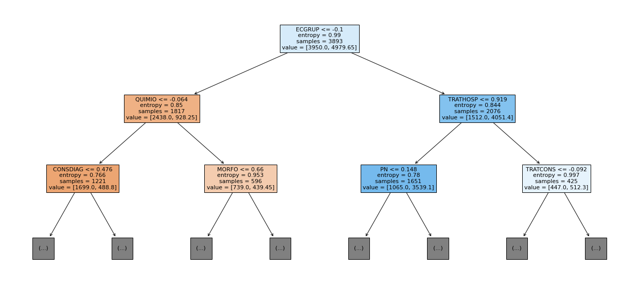
[ ]:
plot_roc_curve(rf_fora_12_15, X_trainOS_12_15, X_testOS_12_15, y_trainOS_12_15, y_testOS_12_15)
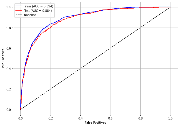
[ ]:
plot_feat_importances(rf_fora_12_15, feat_OS_12_15)
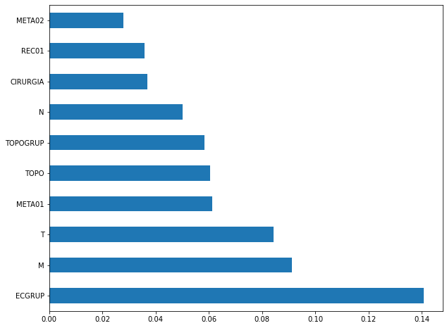
The four most important features in the model were
ECGRUP,M,TandMETA01.
[ ]:
plot_shap_values(rf_fora_12_15, X_testOS_12_15, feat_OS_12_15)
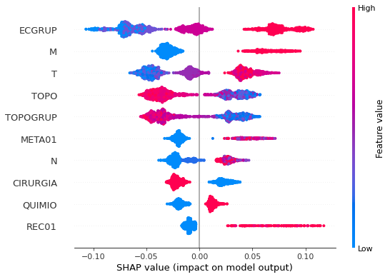
Note that larger values of the ECGRUP column, shown in pink, have more influence for the model’s prediction to be class 1, smaller values have greater weight for the prediction to be class 0. This behavior was expected, because the higher the clinical stage, worse is the stage of cancer.
The other columns shown follow the same logic.
[ ]:
# Other states - 2016 to 2020
rf_fora_16_20 = RandomForestClassifier(random_state=seed,
class_weight={0:1, 1:3.05},
criterion='entropy',
max_depth=8)
rf_fora_16_20.fit(X_trainOS_16_20, y_trainOS_16_20)
RandomForestClassifier(class_weight={0: 1, 1: 3.05}, criterion='entropy',
max_depth=8, random_state=10)
[ ]:
display_confusion_matrix(rf_fora_16_20, X_testOS_16_20, y_testOS_16_20)

precision recall f1-score support
0 0.922 0.815 0.865 1501
1 0.623 0.815 0.706 561
accuracy 0.815 2062
macro avg 0.772 0.815 0.786 2062
weighted avg 0.840 0.815 0.822 2062
The confusion matrix obtained for the Random Forest, with other states data from 2016 to 2020, also shows a good performance of the model, presenting 81% of accuracy.
[ ]:
show_tree(rf_fora_16_20, feat_OS_16_20, 2)

[ ]:
plot_roc_curve(rf_fora_16_20, X_trainOS_16_20, X_testOS_16_20, y_trainOS_16_20, y_testOS_16_20)
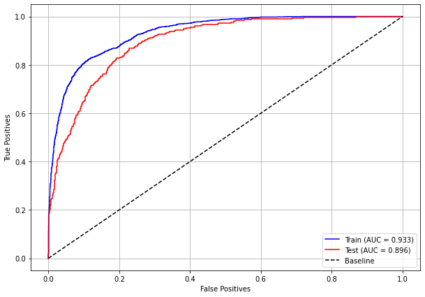
[ ]:
plot_feat_importances(rf_fora_16_20, feat_OS_16_20)
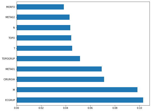
The four most important features in the model were
ECGRUP,M,CIRURGIAandMETA01.
[ ]:
plot_shap_values(rf_fora_16_20, X_testOS_16_20, feat_OS_16_20)
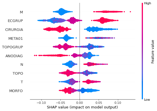
Note that larger values of the M column, shown in pink, have more influence for the model’s prediction to be class 1, smaller values have greater weight for the prediction to be class 0.
The other columns shown follow the same logic.
XGBoost
The training of the XGBoost models follows the same pattern with random_state. The hyperparameter scale_pos_weight was also used in the trainings, in order to obtain a balanced main diagonal in the confusion matrix.
The hyperparameter max_depth was chosen as 10 because the default value for this hyperparameter is 3, a low value for the amount of data we have.
SP
[ ]:
# SP - 2000 to 2003
xgb_sp_00_03 = XGBClassifier(max_depth=8,
random_state=seed,
scale_pos_weight=0.44)
xgb_sp_00_03.fit(X_trainSP_00_03, y_trainSP_00_03)
XGBClassifier(max_depth=8, random_state=10, scale_pos_weight=0.44)
[ ]:
display_confusion_matrix(xgb_sp_00_03, X_testSP_00_03, y_testSP_00_03)

precision recall f1-score support
0 0.632 0.792 0.703 4788
1 0.894 0.791 0.839 10579
accuracy 0.791 15367
macro avg 0.763 0.792 0.771 15367
weighted avg 0.812 0.791 0.797 15367
The confusion matrix obtained for the XGBoost, with the SP data from 2000 to 2003, shows a good performance of the model, here with 79% of accuracy.
[ ]:
plot_roc_curve(xgb_sp_00_03, X_trainSP_00_03, X_testSP_00_03, y_trainSP_00_03, y_testSP_00_03)
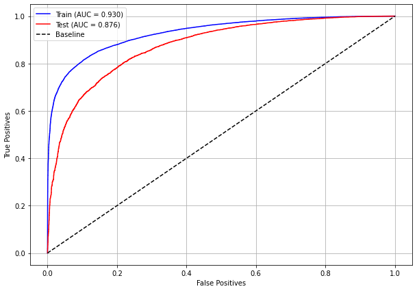
[ ]:
plot_feat_importances(xgb_sp_00_03, feat_SP_00_03)
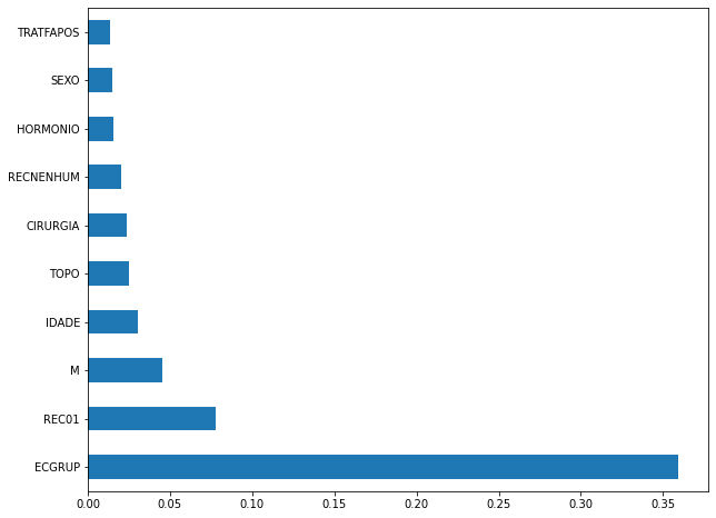
Here we noticed that the most used feature was
ECGRUP, with a lot advantage over the others. Following we haveREC01,MandIDADE.
[ ]:
plot_shap_values(xgb_sp_00_03, X_testSP_00_03, feat_SP_00_03)
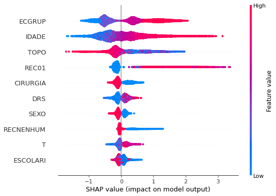
Note that larger values of the ECGRUP column, shown in pink, have more influence for the model’s prediction to be class 1, smaller values have greater weight for the prediction to be class 0. This behavior was expected, because the higher the clinical stage, worse is the stage of cancer.
The other columns shown follow the same logic.
[ ]:
# SP - 2004 to 2007
xgb_sp_04_07 = XGBClassifier(max_depth=8,
random_state=seed,
scale_pos_weight=0.71)
xgb_sp_04_07.fit(X_trainSP_04_07, y_trainSP_04_07)
XGBClassifier(max_depth=8, random_state=10, scale_pos_weight=0.71)
[ ]:
display_confusion_matrix(xgb_sp_04_07, X_testSP_04_07, y_testSP_04_07)

precision recall f1-score support
0 0.718 0.798 0.756 7582
1 0.860 0.799 0.829 11808
accuracy 0.799 19390
macro avg 0.789 0.798 0.792 19390
weighted avg 0.805 0.799 0.800 19390
The confusion matrix obtained for the XGBoost, with the SP data from 2004 to 2007, shows a good performance of the model, with 80% of accuracy.
[ ]:
plot_roc_curve(xgb_sp_04_07, X_trainSP_04_07, X_testSP_04_07, y_trainSP_04_07, y_testSP_04_07)
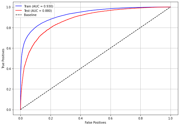
[ ]:
plot_feat_importances(xgb_sp_04_07, feat_SP_04_07)
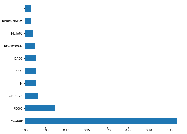
Here we noticed that the most used feature was
ECGRUP, with a good advantage over the others. Following we haveREC01,CIRURGIAandM.
[ ]:
plot_shap_values(xgb_sp_04_07, X_testSP_04_07, feat_SP_04_07)
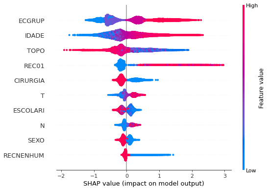
Note that larger values of the ECGRUP column, shown in pink, have more influence for the model’s prediction to be class 1, smaller values have greater weight for the prediction to be class 0. This behavior was expected, because the higher the clinical stage, worse is the stage of cancer.
The other columns shown follow the same logic.
[ ]:
# SP - 2008 to 2011
xgb_sp_08_11 = XGBClassifier(max_depth=8,
scale_pos_weight=1.02,
random_state=seed)
xgb_sp_08_11.fit(X_trainSP_08_11, y_trainSP_08_11)
XGBClassifier(max_depth=8, random_state=10, scale_pos_weight=1.02)
[ ]:
display_confusion_matrix(xgb_sp_08_11, X_testSP_08_11, y_testSP_08_11)

precision recall f1-score support
0 0.795 0.817 0.806 12014
1 0.836 0.816 0.826 13790
accuracy 0.817 25804
macro avg 0.816 0.817 0.816 25804
weighted avg 0.817 0.817 0.817 25804
The confusion matrix obtained for the XGBoost, with SP data from 2008 to 2011, shows a good performance of the model, with 82% of accuracy.
[ ]:
plot_roc_curve(xgb_sp_08_11, X_trainSP_08_11, X_testSP_08_11, y_trainSP_08_11, y_testSP_08_11)
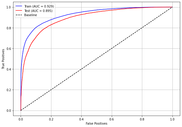
[ ]:
plot_feat_importances(xgb_sp_08_11, feat_SP_08_11)
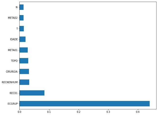
Here we noticed that the most used feature was
ECGRUP, with a good advantage over the others. Following we haveREC01,RECNENHUMandCIRURGIA.
[ ]:
plot_shap_values(xgb_sp_08_11, X_testSP_08_11, feat_SP_08_11)
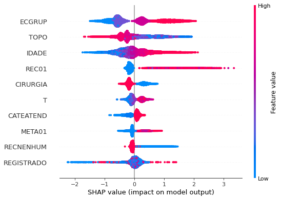
Note that larger values of the ECGRUP column, shown in pink, have more influence for the model’s prediction to be class 1, smaller values have greater weight for the prediction to be class 0. This behavior was expected, because the higher the clinical stage, worse is the stage of cancer.
The other columns shown follow the same logic.
[ ]:
# SP - 2012 to 2015
xgb_sp_12_15 = XGBClassifier(max_depth=8,
random_state=seed,
scale_pos_weight=1.6)
xgb_sp_12_15.fit(X_trainSP_12_15, y_trainSP_12_15)
XGBClassifier(max_depth=8, random_state=10, scale_pos_weight=1.6)
[ ]:
display_confusion_matrix(xgb_sp_12_15, X_testSP_12_15, y_testSP_12_15)

precision recall f1-score support
0 0.867 0.819 0.842 18944
1 0.758 0.818 0.787 13098
accuracy 0.819 32042
macro avg 0.812 0.819 0.815 32042
weighted avg 0.822 0.819 0.820 32042
The confusion matrix obtained for the XGBoost, with SP data from 2012 to 2015, shows a good performance of the model, with 82% of accuracy.
[ ]:
plot_roc_curve(xgb_sp_12_15, X_trainSP_12_15, X_testSP_12_15, y_trainSP_12_15, y_testSP_12_15)
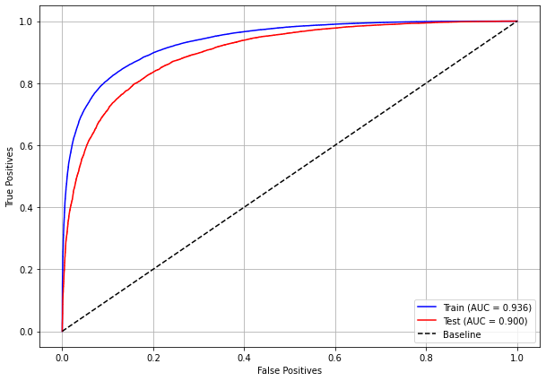
[ ]:
plot_feat_importances(xgb_sp_12_15, feat_SP_12_15)
Here we noticed that the most used feature was
ECGRUP, with some advantage. Following we haveRECNENHUM,REC01andCIRURGIA.
[ ]:
plot_shap_values(xgb_sp_12_15, X_testSP_12_15, feat_SP_12_15)
Note that larger values of the ECGRUP column, shown in pink, have more influence for the model’s prediction to be class 1, smaller values have greater weight for the prediction to be class 0. This behavior was expected, because the higher the clinical stage, worse is the stage of cancer.
The other columns shown follow the same logic.
[ ]:
# SP - 2016 to 2021
xgb_sp_16_21 = XGBClassifier(max_depth=8,
random_state=seed,
scale_pos_weight=2.7)
xgb_sp_16_21.fit(X_trainSP_16_21, y_trainSP_16_21)
XGBClassifier(max_depth=8, random_state=10, scale_pos_weight=2.7)
[ ]:
display_confusion_matrix(xgb_sp_16_21, X_testSP_16_21, y_testSP_16_21)

precision recall f1-score support
0 0.921 0.825 0.871 17508
1 0.656 0.825 0.731 7053
accuracy 0.825 24561
macro avg 0.788 0.825 0.801 24561
weighted avg 0.845 0.825 0.831 24561
The confusion matrix obtained for the XGBoost, for SP data from 2016 to 2021, shows a good performance of the model, with 82% of accuracy.
[ ]:
plot_roc_curve(xgb_sp_16_21, X_trainSP_16_21, X_testSP_16_21, y_trainSP_16_21, y_testSP_16_21)
[ ]:
plot_feat_importances(xgb_sp_16_21, feat_SP_16_21)
The four most important features were
ECGRUP,RECDIST,RECNENHUMandTOPO.
[ ]:
plot_shap_values(xgb_sp_16_21, X_testSP_16_21, feat_SP_16_21)
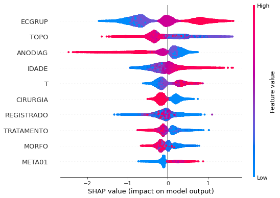
Note that larger values of the ECGRUP column, shown in pink, have more influence for the model’s prediction to be class 1, smaller values have greater weight for the prediction to be class 0. This behavior was expected, because the higher the clinical stage, worse is the stage of cancer.
The other columns shown follow the same logic.
Other states
[ ]:
# Other states - 2000 to 2003
xgb_fora_00_03 = XGBClassifier(max_depth=5,
scale_pos_weight=0.647,
random_state=seed)
xgb_fora_00_03.fit(X_trainOS_00_03, y_trainOS_00_03)
XGBClassifier(max_depth=5, random_state=10, scale_pos_weight=0.647)
[ ]:
display_confusion_matrix(xgb_fora_00_03, X_testOS_00_03, y_testOS_00_03)

precision recall f1-score support
0 0.675 0.769 0.719 334
1 0.841 0.766 0.802 531
accuracy 0.768 865
macro avg 0.758 0.768 0.760 865
weighted avg 0.777 0.768 0.770 865
The confusion matrix obtained for the XGBoost, with other states data from 2000 to 2003, also shows a good performance of the model, with 77% of accuracy.
[ ]:
plot_roc_curve(xgb_fora_00_03, X_trainOS_00_03, X_testOS_00_03, y_trainOS_00_03, y_testOS_00_03)
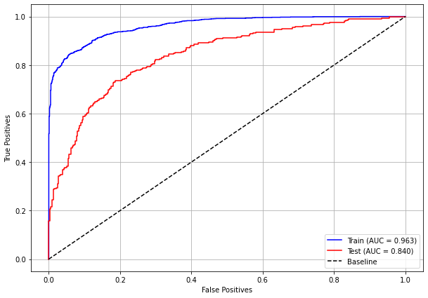
[ ]:
plot_feat_importances(xgb_fora_00_03, feat_OS_00_03)
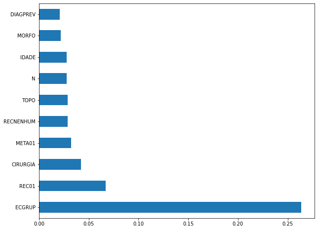
Again we noticed that the most used feature was
ECGRUP, with a good advantage. The following most important features wereREC01,CIRURGIAandMETA01.
[ ]:
plot_shap_values(xgb_fora_00_03, X_testOS_00_03, feat_OS_00_03)
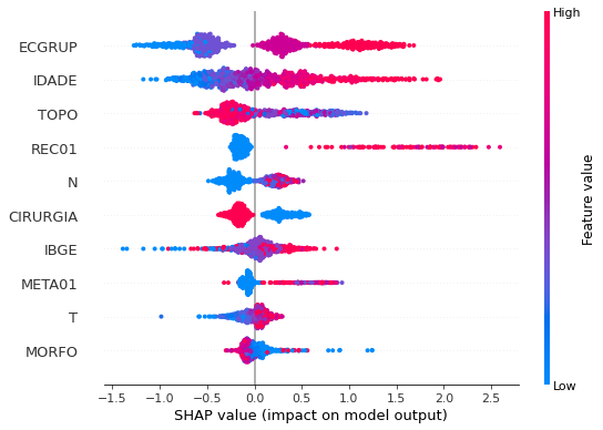
Note that larger values of the ECGRUP column, shown in pink, have more influence for the model’s prediction to be class 1, smaller values have greater weight for the prediction to be class 0. This behavior was expected, because the higher the clinical stage, worse is the stage of cancer.
The other columns shown follow the same logic.
[ ]:
# Other states - 2004 to 2007
xgb_fora_04_07 = XGBClassifier(max_depth=5,
scale_pos_weight=1.032,
random_state=seed)
xgb_fora_04_07.fit(X_trainOS_04_07, y_trainOS_04_07)
XGBClassifier(max_depth=5, random_state=10, scale_pos_weight=1.032)
[ ]:
display_confusion_matrix(xgb_fora_04_07, X_testOS_04_07, y_testOS_04_07)

precision recall f1-score support
0 0.768 0.780 0.774 600
1 0.788 0.777 0.782 632
accuracy 0.778 1232
macro avg 0.778 0.778 0.778 1232
weighted avg 0.779 0.778 0.778 1232
The confusion matrix obtained for the XGBoost, with other states data from 2004 to 2007, also shows a good performance of the model with 78% of accuracy.
[ ]:
plot_roc_curve(xgb_fora_04_07, X_trainOS_04_07, X_testOS_04_07, y_trainOS_04_07, y_testOS_04_07)
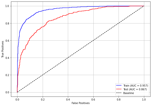
[ ]:
plot_feat_importances(xgb_fora_04_07, feat_OS_04_07)
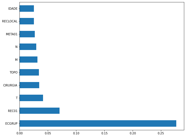
Again we noticed that the most used feature was
ECGRUP, with a good advantage. The following most important features wereREC01,TandCIRURGIA.
[ ]:
plot_shap_values(xgb_fora_04_07, X_testOS_04_07, feat_OS_04_07)
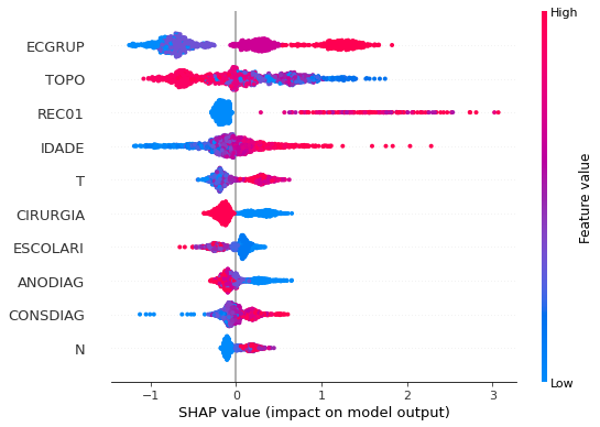
Note that larger values of the ECGRUP column, shown in pink, have more influence for the model’s prediction to be class 1, smaller values have greater weight for the prediction to be class 0. This behavior was expected, because the higher the clinical stage, worse is the stage of cancer.
The other columns shown follow the same logic.
[ ]:
# Other states - 2008 to 2011
xgb_fora_08_11 = XGBClassifier(max_depth=6,
scale_pos_weight=1.28,
random_state=seed)
xgb_fora_08_11.fit(X_trainOS_08_11, y_trainOS_08_11)
XGBClassifier(max_depth=6, random_state=10, scale_pos_weight=1.28)
[ ]:
display_confusion_matrix(xgb_fora_08_11, X_testOS_08_11, y_testOS_08_11)

precision recall f1-score support
0 0.837 0.809 0.823 827
1 0.779 0.810 0.794 686
accuracy 0.810 1513
macro avg 0.808 0.810 0.809 1513
weighted avg 0.811 0.810 0.810 1513
The confusion matrix obtained for the XGBoost, with other states data from 2008 to 2011, also shows a good performance of the model with 81% of accuracy.
[ ]:
plot_roc_curve(xgb_fora_08_11, X_trainOS_08_11, X_testOS_08_11, y_trainOS_08_11, y_testOS_08_11)
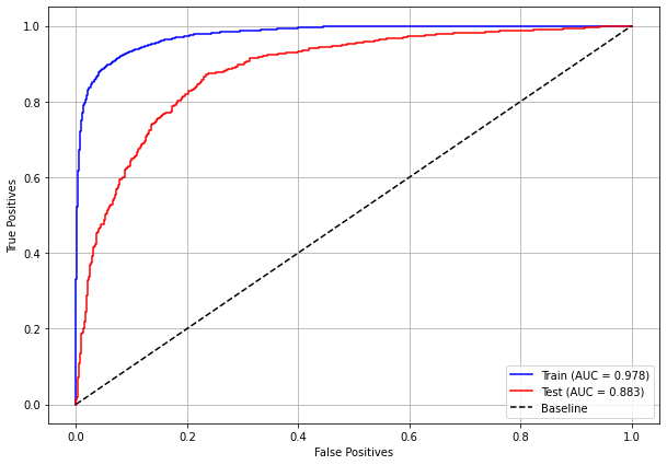
[ ]:
plot_feat_importances(xgb_fora_08_11, feat_OS_08_11)
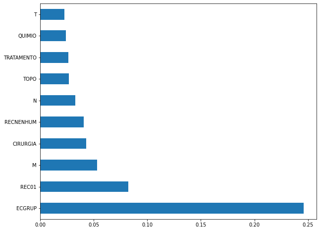
Again we noticed that the most used feature was
ECGRUP, but not with a lot of advantage. The following most important features wereREC01,MandCIRURGIA.
[ ]:
plot_shap_values(xgb_fora_08_11, X_testOS_08_11, feat_OS_08_11)
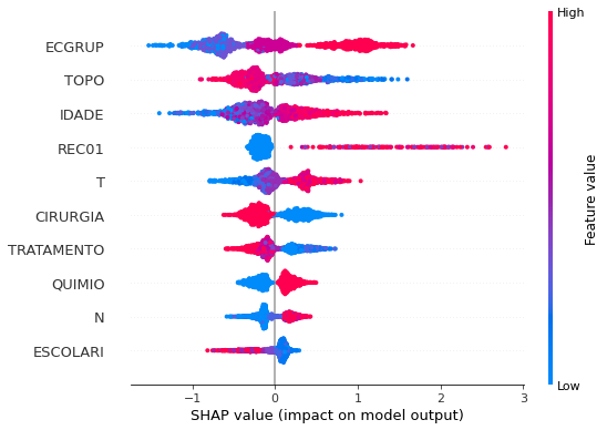
Note that larger values of the ECGRUP column, shown in pink, have more influence for the model’s prediction to be class 1, smaller values have greater weight for the prediction to be class 0. This behavior was expected, because the higher the clinical stage, worse is the stage of cancer.
The other columns shown follow the same logic.
[ ]:
# Other states - 2012 to 2015
xgb_fora_12_15 = XGBClassifier(max_depth=6,
scale_pos_weight=2.65,
random_state=seed)
xgb_fora_12_15.fit(X_trainOS_12_15, y_trainOS_12_15)
XGBClassifier(max_depth=6, random_state=10, scale_pos_weight=2.65)
[ ]:
display_confusion_matrix(xgb_fora_12_15, X_testOS_12_15, y_testOS_12_15)

precision recall f1-score support
0 0.890 0.808 0.847 1327
1 0.689 0.809 0.744 697
accuracy 0.808 2024
macro avg 0.789 0.809 0.795 2024
weighted avg 0.820 0.808 0.811 2024
The confusion matrix obtained for the XGBoost, with other states data from 2012 to 2015, also shows a good performance of the model with 81% of accuracy.
[ ]:
plot_roc_curve(xgb_fora_12_15, X_trainOS_12_15, X_testOS_12_15, y_trainOS_12_15, y_testOS_12_15)
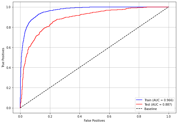
[ ]:
plot_feat_importances(xgb_fora_12_15, feat_OS_12_15)
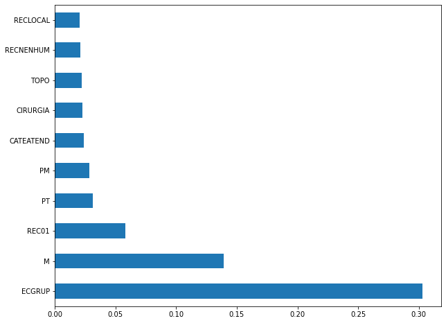
The four most important features were
ECGRUP,M,REC01andPT.
[ ]:
plot_shap_values(xgb_fora_12_15, X_testOS_12_15, feat_OS_12_15)
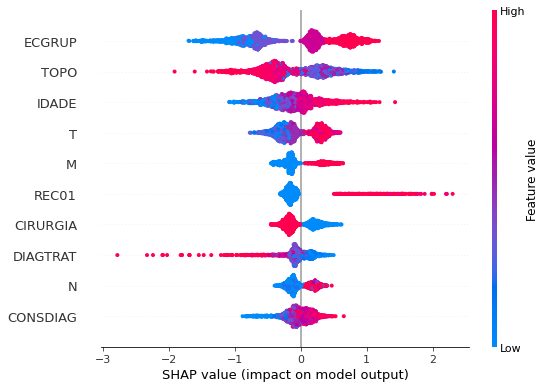
Note that larger values of the ECGRUP column, shown in pink, have more influence for the model’s prediction to be class 1, smaller values have greater weight for the prediction to be class 0. This behavior was expected, because the higher the clinical stage, worse is the stage of cancer.
The other columns shown follow the same logic.
[ ]:
# Other states - 2016 to 2020
xgb_fora_16_20 = XGBClassifier(max_depth=5,
scale_pos_weight=3,
random_state=seed)
xgb_fora_16_20.fit(X_trainOS_16_20, y_trainOS_16_20)
XGBClassifier(max_depth=5, random_state=10, scale_pos_weight=3)
[ ]:
display_confusion_matrix(xgb_fora_16_20, X_testOS_16_20, y_testOS_16_20)

precision recall f1-score support
0 0.921 0.812 0.863 1501
1 0.618 0.813 0.702 561
accuracy 0.812 2062
macro avg 0.769 0.812 0.783 2062
weighted avg 0.838 0.812 0.819 2062
The confusion matrix obtained for the XGBoost, with other states data from 2016 to 2020, shows the best performance comparing with the other models, with 81% of accuracy.
[ ]:
plot_roc_curve(xgb_fora_16_20, X_trainOS_16_20, X_testOS_16_20, y_trainOS_16_20, y_testOS_16_20)
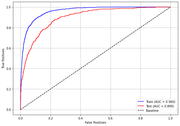
[ ]:
plot_feat_importances(xgb_fora_16_20, feat_OS_16_20)
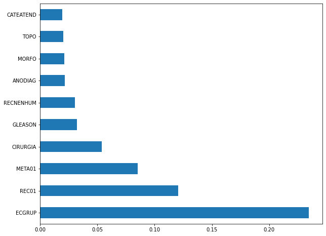
The four most important features were
ECGRUP,REC01,META01andCIRURGIA.
[ ]:
plot_shap_values(xgb_fora_16_20, X_testOS_16_20, feat_OS_16_20)
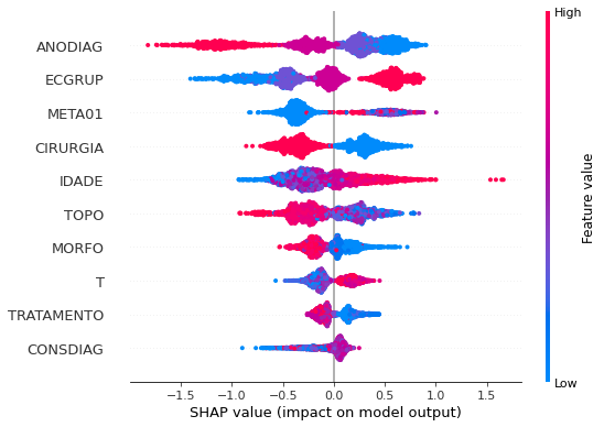
Note that larger values of the ANODIAG column, shown in pink, have more influence for the model’s prediction to be class 0, smaller values have greater weight for the prediction to be class 1.
The other columns shown follow the same logic.
Testing models with data from other years
We will use test data from the following years in the trained models for each set of years grouped together.
Random Forest SP for years 2000 to 2003
[ ]:
display_confusion_matrix(rf_sp_00_03, X_testSP_04_07, y_testSP_04_07)

precision recall f1-score support
0 0.695 0.762 0.727 7582
1 0.837 0.785 0.810 11808
accuracy 0.776 19390
macro avg 0.766 0.774 0.769 19390
weighted avg 0.781 0.776 0.778 19390
[ ]:
display_confusion_matrix(rf_sp_00_03, X_testSP_08_11, y_testSP_08_11)

precision recall f1-score support
0 0.782 0.748 0.765 12014
1 0.788 0.819 0.803 13790
accuracy 0.786 25804
macro avg 0.785 0.783 0.784 25804
weighted avg 0.785 0.786 0.785 25804
[ ]:
display_confusion_matrix(rf_sp_00_03, X_testSP_12_15, y_testSP_12_15)
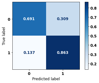
precision recall f1-score support
0 0.879 0.691 0.774 18944
1 0.659 0.863 0.747 13098
accuracy 0.761 32042
macro avg 0.769 0.777 0.761 32042
weighted avg 0.789 0.761 0.763 32042
[ ]:
display_confusion_matrix(rf_sp_00_03, X_testSP_16_21, y_testSP_16_21)

precision recall f1-score support
0 0.944 0.536 0.684 17508
1 0.445 0.922 0.600 7053
accuracy 0.647 24561
macro avg 0.695 0.729 0.642 24561
weighted avg 0.801 0.647 0.660 24561
XGBoost SP for years 2000 to 2003
[ ]:
display_confusion_matrix(xgb_sp_00_03, X_testSP_04_07, y_testSP_04_07)
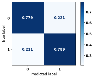
precision recall f1-score support
0 0.703 0.779 0.739 7582
1 0.848 0.789 0.817 11808
accuracy 0.785 19390
macro avg 0.776 0.784 0.778 19390
weighted avg 0.791 0.785 0.787 19390
[ ]:
display_confusion_matrix(xgb_sp_00_03, X_testSP_08_11, y_testSP_08_11)

precision recall f1-score support
0 0.781 0.743 0.762 12014
1 0.785 0.819 0.802 13790
accuracy 0.784 25804
macro avg 0.783 0.781 0.782 25804
weighted avg 0.783 0.784 0.783 25804
[ ]:
display_confusion_matrix(xgb_sp_00_03, X_testSP_12_15, y_testSP_12_15)
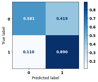
precision recall f1-score support
0 0.884 0.581 0.702 18944
1 0.595 0.890 0.713 13098
accuracy 0.708 32042
macro avg 0.740 0.736 0.707 32042
weighted avg 0.766 0.708 0.706 32042
[ ]:
display_confusion_matrix(xgb_sp_00_03, X_testSP_16_21, y_testSP_16_21)
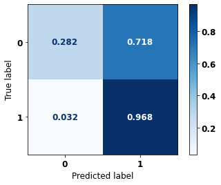
precision recall f1-score support
0 0.956 0.282 0.435 17508
1 0.352 0.968 0.516 7053
accuracy 0.479 24561
macro avg 0.654 0.625 0.476 24561
weighted avg 0.783 0.479 0.458 24561
Random Forest SP for years 2004 to 2007
[ ]:
display_confusion_matrix(rf_sp_04_07, X_testSP_08_11, y_testSP_08_11)
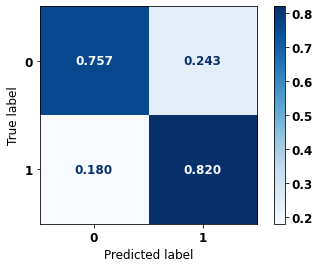
precision recall f1-score support
0 0.785 0.757 0.771 12014
1 0.795 0.820 0.807 13790
accuracy 0.791 25804
macro avg 0.790 0.789 0.789 25804
weighted avg 0.791 0.791 0.790 25804
[ ]:
display_confusion_matrix(rf_sp_04_07, X_testSP_12_15, y_testSP_12_15)
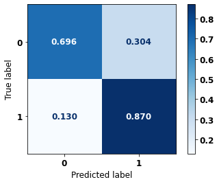
precision recall f1-score support
0 0.886 0.696 0.780 18944
1 0.664 0.870 0.753 13098
accuracy 0.767 32042
macro avg 0.775 0.783 0.766 32042
weighted avg 0.795 0.767 0.769 32042
[ ]:
display_confusion_matrix(rf_sp_04_07, X_testSP_16_21, y_testSP_16_21)

precision recall f1-score support
0 0.948 0.570 0.712 17508
1 0.464 0.923 0.617 7053
accuracy 0.671 24561
macro avg 0.706 0.746 0.665 24561
weighted avg 0.809 0.671 0.685 24561
XGBoost SP for years 2004 to 2007
[ ]:
display_confusion_matrix(xgb_sp_04_07, X_testSP_08_11, y_testSP_08_11)

precision recall f1-score support
0 0.799 0.740 0.769 12014
1 0.787 0.838 0.812 13790
accuracy 0.793 25804
macro avg 0.793 0.789 0.790 25804
weighted avg 0.793 0.793 0.792 25804
[ ]:
display_confusion_matrix(xgb_sp_04_07, X_testSP_12_15, y_testSP_12_15)
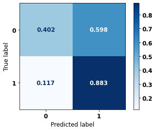
precision recall f1-score support
0 0.833 0.402 0.542 18944
1 0.505 0.883 0.643 13098
accuracy 0.598 32042
macro avg 0.669 0.642 0.592 32042
weighted avg 0.699 0.598 0.583 32042
[ ]:
display_confusion_matrix(xgb_sp_04_07, X_testSP_16_21, y_testSP_16_21)
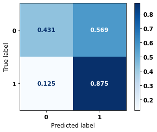
precision recall f1-score support
0 0.896 0.431 0.582 17508
1 0.383 0.875 0.533 7053
accuracy 0.559 24561
macro avg 0.639 0.653 0.557 24561
weighted avg 0.748 0.559 0.568 24561
Random Forest SP for years 2008 to 2011
[ ]:
display_confusion_matrix(rf_sp_08_11, X_testSP_12_15, y_testSP_12_15)

precision recall f1-score support
0 0.872 0.747 0.805 18944
1 0.697 0.841 0.762 13098
accuracy 0.786 32042
macro avg 0.785 0.794 0.784 32042
weighted avg 0.801 0.786 0.788 32042
[ ]:
display_confusion_matrix(rf_sp_08_11, X_testSP_16_21, y_testSP_16_21)

precision recall f1-score support
0 0.952 0.589 0.728 17508
1 0.476 0.926 0.629 7053
accuracy 0.686 24561
macro avg 0.714 0.757 0.678 24561
weighted avg 0.815 0.686 0.699 24561
XGBoost SP for years 2008 to 2011
[ ]:
display_confusion_matrix(xgb_sp_08_11, X_testSP_12_15, y_testSP_12_15)
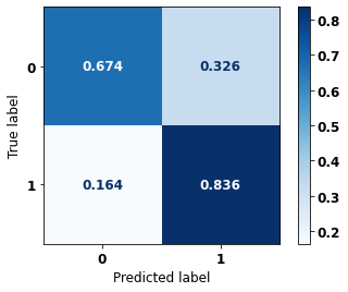
precision recall f1-score support
0 0.856 0.674 0.754 18944
1 0.639 0.836 0.725 13098
accuracy 0.740 32042
macro avg 0.748 0.755 0.739 32042
weighted avg 0.767 0.740 0.742 32042
[ ]:
display_confusion_matrix(xgb_sp_08_11, X_testSP_16_21, y_testSP_16_21)
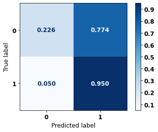
precision recall f1-score support
0 0.918 0.226 0.363 17508
1 0.331 0.950 0.491 7053
accuracy 0.434 24561
macro avg 0.624 0.588 0.427 24561
weighted avg 0.749 0.434 0.400 24561
Random Forest SP for years 2012 to 2015
[ ]:
display_confusion_matrix(rf_sp_12_15, X_testSP_16_21, y_testSP_16_21)

precision recall f1-score support
0 0.927 0.713 0.806 17508
1 0.547 0.861 0.669 7053
accuracy 0.755 24561
macro avg 0.737 0.787 0.737 24561
weighted avg 0.818 0.755 0.767 24561
XGBoost SP for years 2012 to 2015
[ ]:
display_confusion_matrix(xgb_sp_12_15, X_testSP_16_21, y_testSP_16_21)

precision recall f1-score support
0 0.930 0.724 0.815 17508
1 0.559 0.865 0.679 7053
accuracy 0.765 24561
macro avg 0.744 0.795 0.747 24561
weighted avg 0.824 0.765 0.776 24561
Random Forest Other states for years 2000 to 2003
[ ]:
display_confusion_matrix(rf_fora_00_03, X_testOS_04_07, y_testOS_04_07)
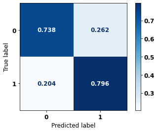
precision recall f1-score support
0 0.774 0.738 0.756 600
1 0.762 0.796 0.779 632
accuracy 0.768 1232
macro avg 0.768 0.767 0.767 1232
weighted avg 0.768 0.768 0.768 1232
[ ]:
display_confusion_matrix(rf_fora_00_03, X_testOS_08_11, y_testOS_08_11)

precision recall f1-score support
0 0.862 0.712 0.780 827
1 0.713 0.863 0.781 686
accuracy 0.781 1513
macro avg 0.788 0.788 0.781 1513
weighted avg 0.795 0.781 0.781 1513
[ ]:
display_confusion_matrix(rf_fora_00_03, X_testOS_12_15, y_testOS_12_15)

precision recall f1-score support
0 0.912 0.656 0.763 1327
1 0.573 0.879 0.694 697
accuracy 0.733 2024
macro avg 0.743 0.768 0.729 2024
weighted avg 0.795 0.733 0.740 2024
[ ]:
display_confusion_matrix(rf_fora_00_03, X_testOS_16_20, y_testOS_16_20)

precision recall f1-score support
0 0.959 0.606 0.742 1501
1 0.469 0.930 0.623 561
accuracy 0.694 2062
macro avg 0.714 0.768 0.683 2062
weighted avg 0.825 0.694 0.710 2062
XGBoost Other states for years 2000 to 2003
[ ]:
display_confusion_matrix(xgb_fora_00_03, X_testOS_04_07, y_testOS_04_07)
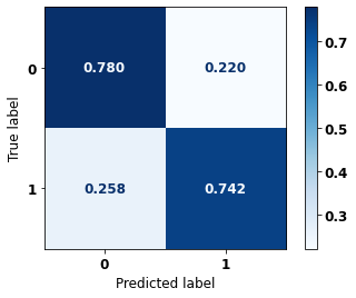
precision recall f1-score support
0 0.742 0.780 0.760 600
1 0.780 0.742 0.761 632
accuracy 0.761 1232
macro avg 0.761 0.761 0.761 1232
weighted avg 0.762 0.761 0.761 1232
[ ]:
display_confusion_matrix(xgb_fora_00_03, X_testOS_08_11, y_testOS_08_11)

precision recall f1-score support
0 0.850 0.751 0.797 827
1 0.737 0.840 0.785 686
accuracy 0.791 1513
macro avg 0.793 0.795 0.791 1513
weighted avg 0.798 0.791 0.792 1513
[ ]:
display_confusion_matrix(xgb_fora_00_03, X_testOS_12_15, y_testOS_12_15)

precision recall f1-score support
0 0.910 0.712 0.799 1327
1 0.613 0.867 0.718 697
accuracy 0.765 2024
macro avg 0.761 0.789 0.758 2024
weighted avg 0.808 0.765 0.771 2024
[ ]:
display_confusion_matrix(xgb_fora_00_03, X_testOS_16_20, y_testOS_16_20)
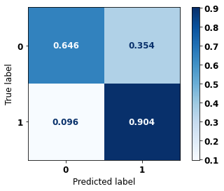
precision recall f1-score support
0 0.947 0.646 0.768 1501
1 0.488 0.904 0.634 561
accuracy 0.716 2062
macro avg 0.718 0.775 0.701 2062
weighted avg 0.822 0.716 0.732 2062
Random Forest Other states for years 2004 to 2007
[ ]:
display_confusion_matrix(rf_fora_04_07, X_testOS_08_11, y_testOS_08_11)

precision recall f1-score support
0 0.856 0.728 0.787 827
1 0.722 0.853 0.782 686
accuracy 0.785 1513
macro avg 0.789 0.790 0.785 1513
weighted avg 0.796 0.785 0.785 1513
[ ]:
display_confusion_matrix(rf_fora_04_07, X_testOS_12_15, y_testOS_12_15)
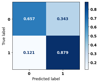
precision recall f1-score support
0 0.912 0.657 0.764 1327
1 0.574 0.879 0.695 697
accuracy 0.734 2024
macro avg 0.743 0.768 0.729 2024
weighted avg 0.796 0.734 0.740 2024
[ ]:
display_confusion_matrix(rf_fora_04_07, X_testOS_16_20, y_testOS_16_20)

precision recall f1-score support
0 0.959 0.614 0.748 1501
1 0.474 0.930 0.628 561
accuracy 0.700 2062
macro avg 0.717 0.772 0.688 2062
weighted avg 0.827 0.700 0.716 2062
XGBoost Other states for years 2004 to 2007
[ ]:
display_confusion_matrix(xgb_fora_04_07, X_testOS_08_11, y_testOS_08_11)

precision recall f1-score support
0 0.861 0.719 0.784 827
1 0.718 0.860 0.782 686
accuracy 0.783 1513
macro avg 0.789 0.790 0.783 1513
weighted avg 0.796 0.783 0.783 1513
[ ]:
display_confusion_matrix(xgb_fora_04_07, X_testOS_12_15, y_testOS_12_15)

precision recall f1-score support
0 0.910 0.657 0.763 1327
1 0.573 0.877 0.693 697
accuracy 0.733 2024
macro avg 0.742 0.767 0.728 2024
weighted avg 0.794 0.733 0.739 2024
[ ]:
display_confusion_matrix(xgb_fora_04_07, X_testOS_16_20, y_testOS_16_20)

precision recall f1-score support
0 0.966 0.593 0.735 1501
1 0.465 0.945 0.623 561
accuracy 0.689 2062
macro avg 0.715 0.769 0.679 2062
weighted avg 0.830 0.689 0.704 2062
Random Forest Other states for years 2008 to 2011
[ ]:
display_confusion_matrix(rf_fora_08_11, X_testOS_12_15, y_testOS_12_15)
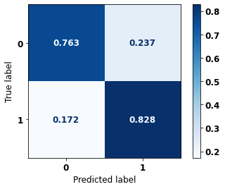
precision recall f1-score support
0 0.894 0.763 0.824 1327
1 0.648 0.828 0.727 697
accuracy 0.786 2024
macro avg 0.771 0.796 0.775 2024
weighted avg 0.809 0.786 0.790 2024
[ ]:
display_confusion_matrix(rf_fora_08_11, X_testOS_16_20, y_testOS_16_20)
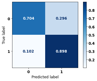
precision recall f1-score support
0 0.949 0.704 0.808 1501
1 0.531 0.898 0.668 561
accuracy 0.757 2062
macro avg 0.740 0.801 0.738 2062
weighted avg 0.835 0.757 0.770 2062
XGBoost Other states for years 2008 to 2011
[ ]:
display_confusion_matrix(xgb_fora_08_11, X_testOS_12_15, y_testOS_12_15)
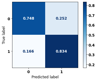
precision recall f1-score support
0 0.895 0.748 0.815 1327
1 0.635 0.834 0.721 697
accuracy 0.778 2024
macro avg 0.765 0.791 0.768 2024
weighted avg 0.806 0.778 0.783 2024
[ ]:
display_confusion_matrix(xgb_fora_08_11, X_testOS_16_20, y_testOS_16_20)
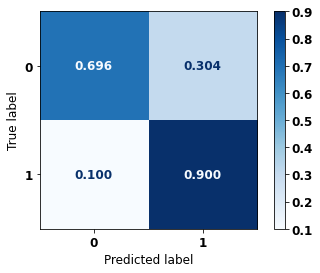
precision recall f1-score support
0 0.949 0.696 0.803 1501
1 0.525 0.900 0.663 561
accuracy 0.751 2062
macro avg 0.737 0.798 0.733 2062
weighted avg 0.834 0.751 0.765 2062
Random Forest Other states for years 2012 to 2015
[ ]:
display_confusion_matrix(rf_fora_12_15, X_testOS_16_20, y_testOS_16_20)

precision recall f1-score support
0 0.941 0.723 0.818 1501
1 0.542 0.879 0.671 561
accuracy 0.765 2062
macro avg 0.742 0.801 0.744 2062
weighted avg 0.833 0.765 0.778 2062
XGBoost Other states for years 2012 to 2015
[ ]:
display_confusion_matrix(xgb_fora_12_15, X_testOS_16_20, y_testOS_16_20)

precision recall f1-score support
0 0.934 0.711 0.807 1501
1 0.528 0.866 0.656 561
accuracy 0.753 2062
macro avg 0.731 0.789 0.732 2062
weighted avg 0.824 0.753 0.766 2062